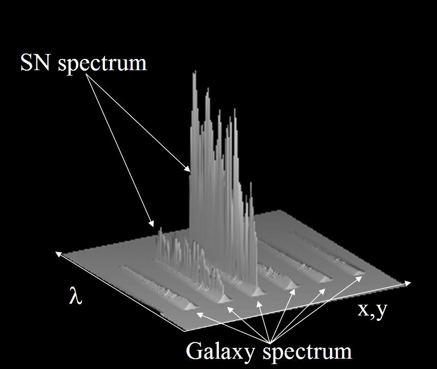
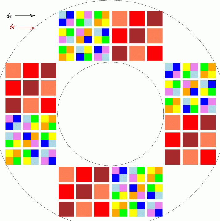
Simulated detector exposure for the observation of a SN and its host galaxy, created with the end-to-end simulator.
Contents
In conventional CCD cameras, "flatfields" make corrections for the pixel-to-pixel variations in sensitivity across a detector. The SNAP focal plane, with its many detectors, is larger and more complicated than ordinary cameras, and so involves additional sources of error. We use the term "flatfielding" to mean "correcting all types of systematic photometric errors across the SNAP focal plane." We also include in this document the additional photometric effects which may occur in the spectrograph at the center of the SNAP focal plane.
In the ordinary "mowing" observational mode, the SNAP spacecraft will measure supernovae repeatedly, but always on the same set of detectors. There could very easily be small, but significant, systematic differences between, say, supernovae detected in column 3 of the East Quadrant and those detected in column 5 of the East Quadrant; or between those measured by column 3 of the East Quadrant and those measured by column 3 of the North Quadrant. These systematic differences, if not corrected, could become a dominant source of error in the cosmological calculations. It is therefore vital that we include in the SNAP operational plan special observations which can be used to characterize the several types of systematic error.
The SNAP spectrometer is an IFU instrument based on "image-slicing" technology. The calibration scenario follows the standard steps of this type of instrument. The SNAP mission requires a well calibrated spectrograph for two reasons: it must measure supernovae over a wide range of magnitudes as part of the science mission, and it must also act in a support role for the imaging camera by measuring reference stars. This means than each potential source of error should be well identified and controlled at a level which is, in general, better than 1%.
Spectrograph topics:
The radiometric calibration of the SNAP spectrometer will be performed following the classical two-step procedure: first a flat-field calibration based on the use of internal sources, and second a spectrophotometric calibration based on the observation of standard stars.
The aim of the flat-field calibration of the instrument is to map the relative, spaxel-to-spaxel [1] response of the instrument as a function of wavelength. Ideally, this calibration should be performed by illuminating the field of view of the instrument uniformly both spatially (uniform illumination) and spectrally (flat spectrum source). In reality, while one can quite often obtain a reasonably uniform illumination of an instrument field of view, it is not possible to have a flat-spectrum source. The flat-field calibration will therefore provide the spaxel-to-spaxel response of the instrument relative to a reference spectrum provided by an internal lamp. As it is usually not possible to place the source before the telescope, this flat-field calibration will only take into account the response of the instrument (including its detector) and not the response of the telescope itself. As the instrument response will change with time (this is especially true for the detectors), it will be necessary to repeat it regularly during the mission. The exact frequency is still TBD.
[1] A spaxel is the name given to a spatial sampling element (by analogy to a pixel). In the case of the SNAP spectrometer, the spatial sampling is made at two different stages in the instrument, depending on the direction. Along the dispersion direction, the sampling is performed by the image-slicer. Perpendicular to it, the sampling is performed by the detector.
To meet the high-level requirements on the mission (in particular the scientific requirements), the instrument shall be flat-fielded with an accuracy better than 1.1 % (1-sigma), assuming that it will be repeated every TBD months. This includes both accuracy of the calibration itself and the changes in the instrument response between two calibrations (assumed to contribute to a level of roughly 0.2 % over TBD months).
Note that this calibration will also make use of the results of the on-ground characterization and calibration campaign of the instrument (including of the detectors), when relevant and possible.
Required observations: The flat-field calibration of the instrument will only be performed using the internal sources of the on-board calibration unit (ideally the one used for the calibration of the imager) and will not use "pointed" observations of celestial targets. Flat-fielding calibration sequences will have to be obtained every TBD months. They can be obtained simultaneously for the two channels of the spectrometer if allowed by the internal sources.
In order to perform the flat-field calibration of the instrument with the requested accuracy, the on-board calibration unit and its sources must fulfill a set of basic requirements. In the following we give a brief overview of these requirements, with a short explanation of their origin. Later on, these requirements will be gathered in a specification document for the on-board calibration unit.
Spatial uniformity (1) – At any wavelength within the useful spectral range of the spectrograph, the uniformity of the illumination provided by the on-board calibration unit shall be better than 1 % (1-sigma, TBC) over the complete field of view of the spectrometer. This requirement aims at minimizing the need and the difficulty of calibrating the distribution of light provided by the on-board calibration unit.
Spatial uniformity (2) – At any wavelength within the useful spectral range of the spectrograph, the uniformity of the illumination of the entrance plane of the spectrometer provided by the on-board calibration unit shall be mappable with a second degree polynomial, with an accuracy better than 0.2 % (1 sigma, TBC). This requirement aims at ensuring that no significant high-spatial-frequency variations of the illumination are present (they could jeopardize the flat-field calibration) and at minimizing the number of positions within the field of view where a standard star will have to be observed.
Spectral smoothness – The spectral gradients in the spectrum provided by the on-board calibration unit at the entrance of the spectrometer for the flat-fielding of the instrument shall be less than TBD percent per TBD nm (1 sigma), over the complete useful spectral range of the spectrometer. This requirement aims at avoiding high-frequency spectral gradients in the input spectrum that will, at best, make the flat-fielding of the instrument difficult and, at worst, make it impossible.
Photon rate – The number of photons per second provided per spaxel by the on-board calibration unit at the entrance of the instrument, when used for its flat-field calibration, shall be large enough to reach a signal to noise larger than 100 in less than 100 s (TBC) for all wavelengths within the useful wavelength range of the instrument. This shall be possible without saturating the detector. This requirement aims minimizing the time spent for the flat-fielding of the instrument (overall operational efficiency of the spectrograph).
Stability (1) – At any wavelength within the useful spectral range of the spectrometer and over its complete field of view, the spatial illumination of the entrance plane of the spectrometer provided by the on-board calibration unit shall be stable to better than TBD % over a duration of TBD months (1 sigma). This requirement aims at minimizing the frequency of the observation of the standard spectrophotometric stars.
Stability (2) – At any wavelength within the useful spectral range of the spectrometer, the average over the complete field of view of the spectrum of the illumination provided by the on-board calibration unit at the entrance of the spectrometer shall be stable to better than TBD % over a duration of TBD months (1 sigma). This requirement aims at controlling the degradation of the illumination over the duration of the mission.
We can also set a set of requirements for the spectrometer itself.
Spectral smoothness – The spectral gradients in the radiometric response of the spectrometer shall be less than TBD percent per TBD nm (1 sigma), over the complete useful spectral range of the spectrometer. This requirement aims at avoiding high-frequency spectral gradients in the instrument radiometric response.
Stability – At any wavelength within the useful spectral range of the spectrometer and over its complete field of view, the radiometric response of the spectrometer shall be stable to better than TBD % over a duration of TBD months (1 sigma). This requirement aims at minimizing the frequency of the flat-field calibrations.
The spectrophotometric calibration of the instrument will be performed by observing standard, spectrophotometric stars, the absolute spectrum of which are accurately known. It will provide us with the absolute and relative radiometric response of each spaxel of the spectrometer at all wavelengths within the useful spectral range of the instrument. By comparing the absolute (i.e. in physical units) spectrum of reference stars with the observed, flat-fielded spectrum obtained with the instrument, the spectrophotometric calibration of the instrument will
The standard stars will be observed at different positions within the field of view to account for changes in the response of the instrument over its field of view, as well as for the non-uniformity of the illumination of the internal sources used for its flat-fielding. It may also be necessary to use a small dithering procedure to average out changes in the diffraction losses as a function of the centering of the star within a given slice.
The accuracy of the spectrophotometric calibration of the instrument shall be better than TBD % (1 sigma) over the complete field of view of the instrument and over its complete useful spectral range. Required observations: The spectrophotometric calibration of the instrument will require "pointed" observations of a set of standard spectrophotometric stars. Each star will be observed at different locations within the spectrometer field of view and it may also be necessary to use a small dithering procedure. These observations will have to be repeated every TBD months.
Knowledge of the absolute spectrum of the standard stars – At any wavelength within the useful spectral range of the spectrometer the absolute spectrum of the spectrophotometric standard stars used for the spectrophotometric calibration of the instrument, shall be know to better than 1 % (1 sigma, TBC). This requirement comes from the fact that a poor knowledge of the reference spectrum used in the spectrophotometric calibration will have a direct impact on the accuracy of all measurements recorded by the instrument.
Spatial uniformity – At any wavelength within the useful spectral range of the spectrometer and over its complete field of view, the radiometric response of the telescope shall be spatially uniform to better than TBD % (1 sigma). This part of the optical path is not included when using the internal sources for the flat-fielding of the instrument. It will not be calibrated and must therefore be controlled.
Stability – At any wavelength within the useful spectral range of the spectrograph and over its complete field of view, the radiometric response of the telescope shall be stable to better than TBD % (1 sigma) over TBD months. This requirement aims at minimizing the frequency of the observation of spectrophotometric standard stars.
Due to the distortion in the spectrograph, the spectra coming from a given spaxel are not straight lines on the detector. This spectrographic stage distortion must be corrected either prior to or at the same time as the wavelength calibration. This will be done by measuring the lateral shift of the spectrum of a point-like continuum source (i.e. typically a star with a continuum as featureless as possible). These measurements are repeated for different locations of the source within the field of view of the spectrometer and they are used to fit an analytical model of the distortion that will be used to predict the distortion for all possible source locations within the field of view.
The accuracy of the spectrographic stage distortion calibration of the instrument shall be better than 0.1 detector pixel (1 sigma, TBC) over the complete field of view of the instrument and over its complete useful spectral range. This includes any relevant stability terms.
Required observations: The calibration of the distortion of the spectrographic stage of the instrument will require "pointed" observations of a star with a relatively featureless continuum (a field with several, well-separated stars would be even better). The observation will be repeated for various source locations within the field of view. Note that the spectrophotometric stars used for the radiometric calibration of the instrument are usually hot and have a very featureless continuum. The exposures obtained for the spectrophotometric calibration of the instrument could therefore be used also for the calibration of the distortion. These observations will be repeated every TBD months.
"Smoothness" of the distortion – The lateral distortion of the spectrographic stage of the instrument (perpendicular to the dispersion direction) shall be smooth enough that, at any given wavelength within the useful spectral range of the instrument, it can be described by a polynomial of degree lower than 5 (function of the position in the field of view) with an accuracy better than TBD detector pixel (1 sigma). This requirement aims at minimizing the number of observations necessary to calibrate correctly the distortion (how many source positions have to be explored before obtaining an accurate description of the distortion).
Stability – For all source positions within the spectrometer field of view, the lateral distortion (perpendicular to the dispersion direction) generated by the spectrographic stage of the instrument shall not change by more than TBD detector pixel (1 sigma) over TBD months. This requirement aims at minimizing the frequency of the distortion calibration observations.
The accuracy of the wavelength calibration of the instrument shall be better than 0.2 detector pixel (1 sigma, TBC) over the complete field of view of the instrument and over its complete useful spectral range. This includes any relevant stability terms.
Required observations: The wavelength calibration of the instrument will not require "pointed" observations; it will use dedicated line sources that will be present in the on-board calibration unit. They will have to be repeated every TBD months. Depending on the availability of line sources suitable for the complete wavelength range, the wavelength calibration of the two channels of the spectrograph could be performed simultaneously.
In order to perform the wavelength calibration of the instrument with the requested accuracy, the on-board calibration unit and its sources shall fulfill a set of basic requirements, which are different from those inferred for the flat-field calibration.
Spectral lines (1) – The line source(s) of the on-board calibration unit shall provide a minimum of 20 (TBC) well-separated, high-contrasts line over the complete useful wavelength range of the instrument. This requirement aims at ensuring that the number of lines that will be used as references for the wavelength calibration of the instrument is large enough to ensure an accurate determination of the calibration relation over the complete useful wavelength range of the instrument.
Spectral lines (2) – The line source(s) of the on-board calibration unit shall have FWHM (full width at half maximum) smaller than 15 (TBC) detector pixels. This requirement aims at making sure that the lines (that can be spectrally resolved) are not too large.
Spectral lines (3) – The line source(s) of the on-board calibration unit shall have peak intensities (inferred from their integrated flux and their FWHM assuming a simple Gaussian profile) differing by no more than a factor 5 (TBC). This requirement aims at making sure that in order to reach a minimum signal to noise of 100 on the peak of a given line, we do not saturate any other line (i.e. all lines can be used for the wavelength calibration).
Spatial uniformity – At any wavelength within the useful spectral range of the spectrograph, the uniformity of the illumination provided by the on-board calibration unit when using "line" sources shall be better than 10 % (1 sigma, TBC) over the complete field of view of the spectrometer. This requirement aims at ensuring that, for a given integration time, there are no significant differences in signal to noise on within the field of view due to the non-uniformity of the illumination provided by the on-board calibration unit. Note that this requirement is automatically fulfilled if the on-board calibration unit fulfills the equivalent requirement for the flat-field calibration of the instrument.
Photon rate – The number of photons per second provided per spaxel by the on-board calibration unit at the entrance of the instrument, when used for its wavelength calibration, shall be large enough to reach a peak signal to noise larger than 100 in less than 20 s (TBC). This shall be possible without saturating the detector at any wavelength within the useful spectral range of the instrument. This requirement aims at ensuring that the signal to noise on the lines is high enough to accurately measure their centroid and also that it is obtained quickly enough (the need for long calibration exposures would reduce the overall operational efficiency of the spectrometer).
Stability and knowledge of the position of the lines – At any time during the mission, the intrinsic central wavelength of a given line used for the wavelength calibration of the instrument shall be know to better than 1/40th of a detector pixel (1-sigma, TBC). This requirement is easily and automatically fulfilled for an emission-line source (classical Neon lamp as an example) but this may not be the case for other types of "line" sources.
We can also set a set of requirements for the spectrometer itself.
Smoothness of the calibration relation – The calibration relation (relation providing the wavelength as a function of position in a spectrum) of the spectrometer must be (spectrally) smooth enough so that, for any spaxel and over the complete useful spectral range of the instrument, it can be described by a polynomial of degree lower than 5 (TBC) with an accuracy better than 0.02 detector pixels (1 sigma, TBC). This requirement aims at making sure that the requested number of lines for the sources is high enough to accurately constrain the fit of the calibration relation for all spaxels.
Stability – At any wavelength within the useful spectral range of the spectrometer and over its complete field of view, the calibration relation (relation providing the wavelength as a function of position in a spectrum) of the spectrometer shall be stable to better than TBD % over a duration of TBD months (1 sigma). This requirement aims at minimizing the frequency of the wavelength calibrations.
It is currently thought that the SNAP spectrometer will use the same on-board calibration unit than the imager. However, the spectrometer has needs that can be very different from the ones of the imager. It is therefore necessary to make sure the on-board calibration unit can be used both for the imager and the spectrometer. In the previous sections, we identified requirements on the on-board calibration unit originating from various calibrations. In the following we discuss the impact of some of them on various characteristics of the on-board calibration unit, in particular its sources.
When discussing the flat-field calibration of the spectrometer, we have identified a very stringent requirement on the uniformity (less than 1 %) and smoothness of the illumination provided by the on-board calibration unit at the entrance of the spectrometer. It is not yet clear if the current design of the on-board calibration unit allows meeting this requirement (it is a stringent requirement but it applies to a very small field of view compared to that of the imager). At the end, this may push toward the use of an integrating sphere if possible.
We have also identified a set of requirements for the sources that will be used for the flat-field calibration of the instrument. One major difficulty is probably the need to have a fairly uniform photon rate over such a large wavelength domain (we want to be able to reach a good signal to noise in the dimmest parts of the spectral range without saturating the brightest ones). It is not yet clear if this is possible with a classical tungsten-filament lamp or if it will be necessary to use LEDs (Light Emitting Diodes). In particular, to be able to use tungsten filament lamps in the blue, it is necessary to use high filament temperatures and this may strongly degrade their stability and decrease their lifetime. The final solution may be to use a combination of different lamps and LEDs. It is not clear yet if it will be possible to use the same sources than the imager (this would of course be the ideal scenario).
The need of "line" sources is clearly specific to the spectrometer and is not present for the imager. It will therefore be necessary to have dedicated sources for the wavelength calibration. We have identified a set of different possible solutions for these line sources:
The spectrograph is placed on the back side of the focal plane and the entrance pupil is in the middle of the focal plane. The baseline for the calibration is to use the same on-board calibration unit as the imager. However, we have identified some caveats to be solved. Ensure first an illumination of the entrance of the spectrograph (which is not the case actually) and secondly ensure than the imager lamps fulfill the requirements mentioned above. If this solution is implemented, we can also study the implementation of the lines sources in front of the illumination system.
If it is not possible, we propose to have an internal calibration unit for the spectrometer, using a screen shutter to project the light in the spectrometer. In this case, the spectrometer will have an independent calibration unit for both flat fielfing and wavelength calibration.
In order to cover the complete spectral range running from 0.3 to 1.7 microns, the SNAP spectrometer will have two different arms and will use a dichroic to divert light to each channel. There will be a small overlap region between the blue and red channels of the instrument. The exact location of this region that is foreseen to be somewhere between 0.8 and 1.1 microns is still TBD. It will mainly depend on the properties of the detectors, namely the fringing and efficiency toward the red for the visible detectors and the efficiency toward the blue for the infrared detectors.
It has however already identified that a good radiometric calibration of this overlap region will be needed to make sure we have consistent radiometric measurements between the blue and red channels. Indeed, the transmission curve of the dichroic can display oscillations in the overlap region. These oscillations will typically get stronger if the transition is sharp and they could harm the radiometric calibration of the two channels in this region.
When acquiring scientific exposures and for most calibrations, the spectrometer will not require any shutter and will make use of a so-called "electronic shutter". This is implemented in two very different ways in the blue (visible) and red (infrared) channels of the spectrometer. In the visible (CCD detector) we will use frame-transfer techniques to move the charges into a non-illuminated region of the detector at the end of the exposure. In the near-infrared (IR-type detector), each pixel in the detector will be read out continuously, so there are no spatial variations in sensitivity imposed by changing the exposure time.
These types of "electronic shutters" are appropriate for the long exposure times foreseen for the scientific operation of the instrument. However two others specific needs have been identified that cannot be fulfilled with the current "electronic shutter" baseline.
Measurement of the dark current – we need to guarantee that no photons reach the detectors during this measurement. This requires an external shutter. No special constraints are required either on its speed (it can be very slow) or on the reproducibility of its exposure time. A possible extension of the shutters implemented at the Cassegrain focus of the telescope for the imager can be studied and would probably be adequate. Another solution is an internal shutter for the spectrograph but it would add a mechanism. Radiometric calibration of the fundamental spectrophotometric standard stars -- In the initial phase of the mission, the SNAP spectrometer can be used to transfer the calibration from Vega (magnitude 0) to fundamental standards (magnitude of order 12-15) and then to primary stars (magnitude 16-19), to establish a catalog of calibrators for the imager. It increases the dynamic range the spectrometer needs to accommodate and will require very short exposure times at the level of milliseconds. Dedicated electronic shutters, running under special modes, can be implemented. Preliminary studies show that the required precision can be achieved. This need to be tested more precisely by conducting specific studies using lab prototypes (as planned during the R&D period).
A simulation has been implemented in the SNAP JAVA framework with the simulation group. It is a full simulation of the optical system based on Fourier optics. It is coupled to the detailed design of the instrument via Zernike coefficients produced by the Zemax optical design program. A parameterization based on shapelets decomposition of the PSF has been developed. Shapelets coefficients are interpolated on a continuous grid using a neural network.
The output is a discrete PSF at the detector level, for a monochromatic point source at a given position within the field of view. It can be used to simulate a complete SN spectrum in the range 0.35-1.7 microns, and to verify that the expected performances can be reached. In particular all optical losses or defects can be implemented and their effects evaluated in a complete way.
Simulated detector exposure for the observation of a
SN and its host galaxy, created with the end-to-end simulator.
We are preparing a demonstrator for 2006, focusing on the optical performances of the image slicer and on the validation of the calibration concept for this type of IFU. We plan to test it not only in the visible, but also in the NIR using a Rockwell detector.
The demonstrator will allow us to:
The demonstrator is currently being designed and we will start manufacturing at the end of the year.
In addition there is on-going work on the detectors that may have a significant impact on the calibration concept: the actual detector properties will have a significant impact on the instrumental parameters and the removal of the detector signatures will also depend on the actual detector properties. The baseline is to use a LBNL CCD detector for the visible arm and a Rockwell HgCdTe detector for the infrared arm. We describe here briefly several physical effects that will have to be investigated and monitored thoroughly before and during flight.
Remanence -- The choice of the operating temperature will imply a trade-off between the dark current level and the remanence effects after an intense illumination. Our forthcoming tests will evaluate quantitatively the temperature dependence of the remanence. As the fluxes are lower in the spectrograph, the nominal choice of operating temperature might be different than for the imager.
Non linearity -- We do not anticipate any specific problem in the evaluation of the non linearity of the detector and readout electronic responses. The possibility of distinguishing both contributions would imply the inclusion of a test signal on some of the reference unconnected pixels. These pixels may be less suitable for the common mode noise subtraction if such a configuration is implemented. Light signals of varying duration seem the easiest way of ensuring a linear variation, but monitoring photodiodes would help control secondary effects, such as an increased temperature for longer signals.
Fringing -- It is assumed at present that the CCD thickness is limited to 100 microns in the spectrograph, in order to lower the number of pixels affected by a cosmic ray impacts. Some residual fringing oscillation might still be observed beyond 0.8 microns. This will have to be measured during the ground tests of the spectrometer. The fringing corrections may require a detailed understanding of the detector, as shown in the HST analysis. Given the complexity of implementing fringing corrections, the level of fringing of a given detector will be an important consideration in the choice of the location (in wavelength) of the overlap region between the blue and red channels of the spectrograph.
Some specific programs for testing detectors both in the visible and the NIR will be conducted, (mainly in US, by the GSFC group). They will do some specific trade off studies:
The variations in response across the SNAP focal plane, or the "flat-field", is typically characterized by two components: small-scale pixel-to-pixel variations, or "high-frequency spatial flats", and large-scale variations, or "low-frequency spatial flats". High spatial frequency variations are usually introduced by individual pixel response differences and by shadows created by particulates deposited on filters or the CCD itself. To correct for these pixel-to-pixel variations, the focal plane is often illuminated with diffuse light that is spatially uniform, or "flat", so that the individual pixel responses can be normalized one to the other.
In ordinary astronomical observations, the diffuse irradiance is usually provided by a lamp source reflected off the dome (dome flat) or the twilight sky (twilight flat). For SNAP, the Ring of Fire (RoF) functions as the diffuse source of irradiance. As shown below, the RoF places a series of lamp sources around the entrance to the cold stop. These lamps irradiate a ring of diffuse reflecting material along the opposite wall of the cold stop that scatters light onto the focal plane in a well-characterized azimuthal and radial pattern. There are several advantages to such a system. By using accurately calibrated lamp sources, the flat field irradiance can be characterized to high precision, thereby yielding very accurate high spatial frequency flat fields (monitoring the irradiance for variations with photodiodes will be discussed later).
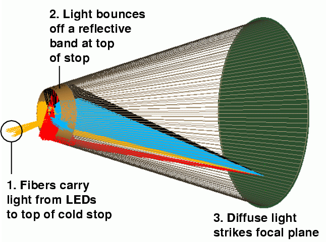
The Ring of Fire (see Scholl 2004 for a full description).
Similar high precision high frequency flat fields can be obtained by dithering well-characterized calibration stars over the focal plane. But the large number of pixels on the SNAP focal plane, roughly half a billion, makes this approach very costly in time. There are also other significant advantages to the RoF. First, high frequency flat fielding can done routinely and quickly. Second, the RoF incorporates lamp sources with well-calibrated irradiance that are monitored by NIST-calibrated photodiodes. The RoF thus provides an accurate absolute flux scale for the SNAP photometry. Third, the calibrated irradiance on the focal plane from the RoF provides a means to monitor variations in the filters, as well as standard tests of detector performance.
However, the RoF does have a disadvantage when compared with standard flat-fielding techniques. While the RoF delivers calibrated diffuse light to the focal plane on small chip scales, SNAP does not currently have a scheme that puts this irradiance though the entire SNAP optical train. On the other hand, changes in the flat field due to the SNAP mirror assembly should be seen over large-scales and can therefor corrected with "star-flats" (discussed later) and with "super-flats" created from observations of the zodiacal light background.
The RoF presents some interesting challenges. Ideally, the RoF is designed to illuminate the focal plane with calibrated irradiance. Traditionally, QTH (Quartz Tungsten Halogen) lamps have been used in this role. It is not possible, however, to mount several QTH lamp sources at that position with the space constraints at the entrance to the cold stop. In addition, QTH lamps have shown that the difference in gravitational loading between ground calibration and space can change the irradiance of the lamp significantly. We plan to remedy this situation by using pulsed LEDs to illuminate fiber optics which deliver light to the RoF. LEDs are solid state devices that will be more stable on orbit than QTH lamps and can have controlled light output if pulsed on a low-duty cycle. LEDs also can be manufactured with a large number of narrow wavelength ranges from the optical to the near infrared which will be useful in calibrating detectors and filters.
Coupled with calibrated photodiodes on the SNAP focal plane to monitor the irradiance, the RoF will yield a steady source of irradiance that can correct small-scale flux variations, as well as monitor system response.
A single detector will often have significant large-scale variations in its quantum efficiency. By "large-scale", I mean "over many tens or hundreds of pixels", or "over signficant fractions of its entire extent." In addition to any which are intrinsic to the device, we will add this sort of variation when we divide images by the lamp flatfield images.
We can use "starflats" to identify these errors. The basic idea, as described by Manfroid (1995) or van der Marel (2003), is to take a series of exposures of a starfield, moving the telescope in a grid pattern so that each star is measured at many locations on a single chip. One can fit a model to the variations in observed magnitude as a function of position.
Manfroid states that a 3x3 or 4x4 grid of measurements of a field of 10-20 stars yields excellent results. On the SNAP focal plane, each detector subtends roughly 0.01 square degrees. Using counts of stars near the SNAP North field, we calculate the following cumulative statistics for number of stars falling on a single detector or filter (the optical CCDs may have 4 filters covering the quadrants of a single chip):
                       stars               stars
     V mag range       per chip       per filter (1/4 chip)
     ---------------------------------------------------------
     14.0 - 17.0         7                   2
     15.0 - 18.0        11                   3
     16.0 - 19.0        15                   4
     17.0 - 20.0        22                   6
     18.0 - 21.0        35                   9
     19.0 - 22.0        60                  15
     20.0 - 23.0        89                  22
     ----------------------------------------------------------
If we require 20 stars per chip (filter) to appear in a typical grid image, this suggests we concentrate on stars in the range from V = 17-20 (20-23). Calculations of the signal-to-noise ratio in SNAP images indicate that a star of magnitude V=20 will have S/N=100 in an exposure of roughly 100 seconds.
To first order, the variations we consider here should not depend strongly on stellar color.
Required observations: a series of exposures while moving the telescope over a grid (say, 4x4 or 5x5 positions) which covers a single chip; another set of grid exposures which move stars over a single filter covering one quadrant of an optical CCD.
We can expect each chip to have a slightly different overall quantum efficiency due to variations in the manufacturing process, especially if devices are taken from different lots. As a star moves from one detector of a given sort to another, its observed magnitude will therefore jump by some small amount.
We can determine these variations simply by moving stars from one detector to another of the same sort: that is, from an optical CCD with filter 2 to another optical CCD with filter 2. Note that this requires both relatively short offsets -- for detectors within the same quadrant of the focal plane -- and large offsets -- for detectors in different quadrants.
To first order, we may treat these corrections as independent of stellar color.
Required observations: a series of exposures while moving the telescope so that stars move from one detector to all the others of the same sort.
Current designs call for four mechanical shutters near the Cassegrain focus of the telescope; see the Cassegrain Shutter document (Jelinsky 2004). Each shutter would open to allow light to reach one of the four quadrants of the focal plane. As the shutter blade rotates open, it exposes to light the inner portion of the focal plane for a slightly longer time than the outer portion. This leads to exposure times which vary across the focal plane.
Because the shutter blades move quickly (in roughly 50-80 milliseconds), this effect is significant only for short exposure times, less than 10 or 20 seconds. Jelinsky notes that it is possible to design a system to measure the motion of the blades very accurately, to within 1 millisecond, so that one could make accurate corrections with a good optical model. There are two routes one can take here:
Jelinsky (2004) and Lampton (2003, 2004) describe both methods in some detail. It seems reasonable to do both: calculate the expected variation based on the design, and then check it once in orbit.
The effect is largest for short exposures. Consider a 1-second image: calculations indicate that stars of magnitude V=15 will yield a S/N ratio of 100-300 (highest for red stars measured on the infrared detectors). Most of the stars in the SNAP North field at this magnitude will be of spectral type G and K, which yield S/N approximately 100 in all filters; this corresponds to scatter of about 1 percent from one image to the next. Jelinsky suggests that the size of the shutter effect will be roughly 5 percent for a 1-second exposure. Thus, stars of magnitude V=15 and perhaps a bit fainter should show the effect clearly above random noise. Each shutter blade covers a single quadrant of the focal plane, which contains 18 detectors; each detector subtends roughly 0.01 square degrees, so a quadrant samples about 0.18 square degrees. In the magnitude range V=14 to V=17, we expect roughly 130 stars to be detected on each quadrant. This appears sufficient to measure the shutter effect empirically to high precision.
Required observations: a series of exposures with lengths running over a large range; say, 0.5, 1, 2, 3, 5, 10, 20, 50, 100, 200, 300 seconds. The telescope should remain fixed at one pointing during the series; it may also be possible to use a set of images with very small dithers of a few arcseconds for this purpose.
Although we will provide a clear specification for the SNAP filters, it is possible that small deviations may occur during the manufacturing process. Even if we measure the filters precisely before launch, it is possible that the passbands may shift somewhat after launch, or over the lifetime of the entire mission. How would these changes in effective passband affect the photometry of stars?
We may approximate such deviations from the fiducial passbands as shifts in central wavelength. A study of passband shifts shows there is a clear pattern in the errors such shifts will produce in stellar photometry. The pattern is:
    Type of         As central wavelength of filter shifts
    star               blueward                 redward
    --------------------------------------------------------
     hot blue         grow brighter            grow fainter

     cool red         grow fainter             grow brighter
    --------------------------------------------------------
The amplitude of these changes is largest in the bluest filters of the optical CCDs and smallest in the infrared filters.
We can look for
Required observations:
If the SNAP filters depend on interference rather than colored glass, there will be significant shifts in the bandpass as a function of the angle with which light strikes the filters. From the inner edge to the outer edge of the focal plane annulus, this angle of incidence varies from about 0.14 to 0.28 radians. How will this affect measurements of stars?
Our analysis indicates a simple pattern that should appear as stars move radially away from the center of the focal plane: blue stars grow brighter, and red stars grow fainter. Therefore, one can characterize this effect by taking a series of images and looking at the change in instrumental magnitude as a function of stellar color and distance away from the center of the focal plane.
Required observations: a series of exposures in which stars move (radially) across a single filter, and (radially) from one instance of a filter to another instance of the same filter. Look for changes as a function of stellar color.
It is possible that the optics may cause small differences in illumination on very large scales across the focal plane; we might call such effects "vignetting." Note that such effects could not be detected using images of the internal lamps, since that light does not pass through the optics.
Preliminary estimates are that any such effects would depend only very weakly on the wavelength of light, and hence only very weakly on stellar color. We believe that these very large-scale variations would be removed by the application of corrections already mentioned; specifically,
Required observations: None.
We end up with the following list of stellar exposures to determine "flatfield" corrections:
We plan to make these special observations at the start of the mission and periodically thereafter.
The previous section describes a series of special calibration exposures which should be made at the start of the mission and periodically thereafter. For the bulk of the time, however, the SNAP telescope will execute its normal program of repeatedly scanning a small region of the sky. Let us consider briefly the details of this procedure: is there a "best" way to move the telescope across the sky?
There are two main issues we can address in designing the slewing procedures:
First, let us discuss dithering.
The following discussion assumes that we can control the telescope well enough to point it to a particular sub-pixel location reliably. If that is not the case, then we should simply command the telescope to move by a pixel or so between each exposure and take whatever random dithering we get. We will have enough stars on each detector to extract the exact offset of each sub-exposure from the others after the fact.
The regular observations will involve multiple exposures at each position. As HST and other space-based telescopes have shown, cosmic rays strike a significant fraction of the pixels in a detector over periods of just a few hundred seconds. In order to reach supernovae of magnitude 25 or so with decent signal-to-noise ratios, SNAP must collect light for about 1000 to 1500 seconds. It therefore makes sense to follow the practice of HST and break up the total exposure into several pieces: say, four images, each of 300 seconds. Note that at exposure times of several hundred seconds, noise from the background sky (mostly zodical light) will roughly equal the readout noise for optical CCDs. Readout noise will exceed the background sky noise for the current (May 2005) versions of infrared detectors until the exposure time reaches several thousand seconds. Finally, breaking each exposure into several pieces increases the dynamic range of the dataset, since brighter stars will be recorded without saturation on the shorter individual exposures.
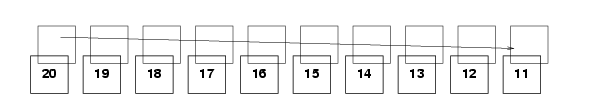
How should we dither the telescope from one sub-exposure to the next? Several scientists have studied the issues involved in sub-pixel dithering. Lauer (1999) finds that moving in a regular NxN grid-like pattern is best for photometry. Bernstein (2002) concludes that a 3x3 grid is nearly always sufficient to recover the original properties of point sources. Suppose that we make one set of four exposures using small offsets of size one-third of a pixel each time:
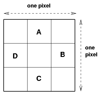
Each individual star will sample only about half of the 3x3 intra-pixel grid during this procedure. However, there will be tens or hundreds of stars on each chip with good signal-to-noise. These stars will be scattered at random across the sub-pixel locations, so that some stars will fall into those other sub-pixel locations:
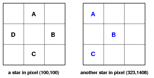
If we assume that the manufacturing process causes the same pattern of intra-pixel sensitivity across each detector, then we can use the many stars measured on each chip in a single set of four sub-exposures to sample all locations in a 3x3 sub-pixel grid.
We now consider a second aspect of telescope motion: the large-scale slews which point the telescope to all portions of the study area, which we denote as the "mowing" pattern.
Because detectors do not cover the entire focal plane, there will be small gaps in the sky coverage between each set of images. For simplicitity's sake, let us illustrate the issue with just two stars, and focus on their motion relative to the top left quadrant of the focal plane during a single pass of the mowing:
If we move the telescope in a straight line across the sky, then it will miss all stars which fall in the gap between two rows of the camera. The gap is roughly 18% of the width of each detector, so each of these linear passes will detect only 82% of the stars in a region.
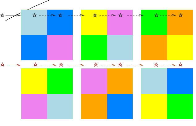
In order to cover a contiguous region, the telescope must make at least two passes. The second pass must involve a shift perpendicular to the scan direction by an amount sufficient to move stars from the inter-row gap to the detectors, like so:
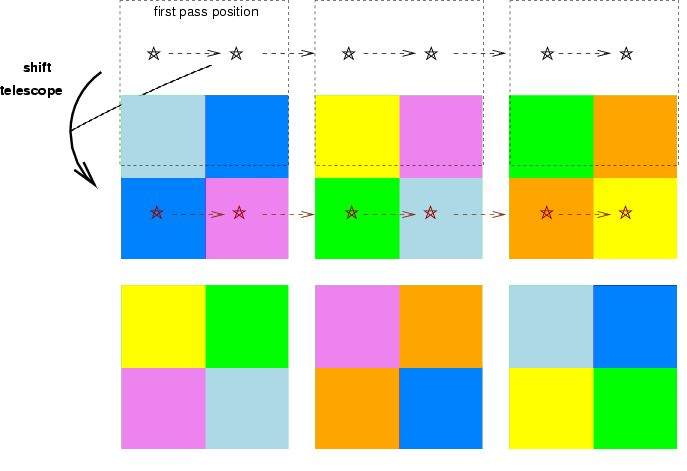
However, there is another gap to consider: the space between two detectors in the scan direction. There are several options to handle this gap. We may choose to slew the telescope along the scan direction in alternating short and long jumps, so that a given star will always appear in the same location within each filtered section of a CCD detector. This will ensure that during one pass of the telescope, many objects will be measured through every filter.
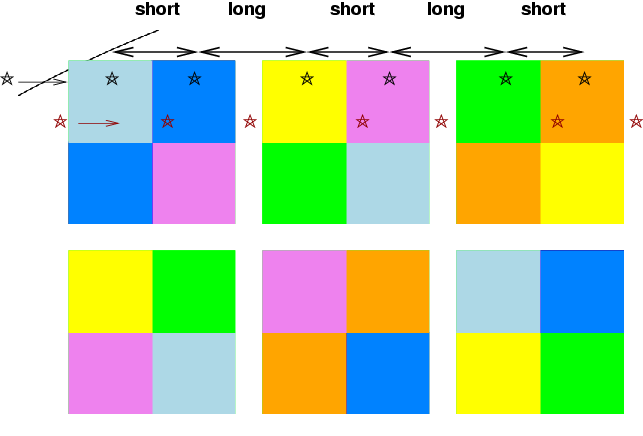
But, as the figure above shows, other objects will repeatedly fall into the gaps between detectors in a row. In order to measure every object through every filter, we must again plan a second pass, this time shifting the telescope's position parallel to the scan direction.
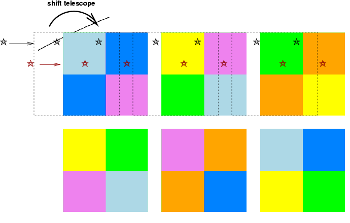
The second pass will involve an offset in both directions from the starting point of the first pass. Since the gaps between columns of detectors are roughly the same size -- about 18% of the detector size -- the yield of two passes with this staggered offset will be
One way to proceed, then, is to make two passes through the survey region. Each pass will consist of pairs of alternating short and long jumps in the scan direction. After completing one pass, the telescope should return to the starting point, offset itself by a fraction of the detector size in both directions (parallel to and perpendicular to the scan), then make another series of short and long jumps as it moves down the region a second time. We suggest this pattern -- go all the way to the end of the survey region in a straight line,
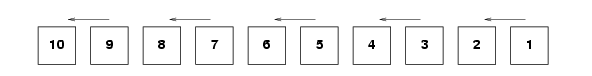
then return for a second long pass,
rather than a zig-zag pattern
because the first method provides better time coverage of the doubly-measured objects than the second. For example, if a star falls onto the detectors in each pass, we will acquire for it
Note that if it is possible to position the telescope at desired sub-pixel locations with some accuracy, we should make the offset between the first and second passes not an integer number N of pixels in each direction, but an integer plus a fraction N + 1/3. In this way, during the second pass, each sub-exposure can fall on a different sub-pixel then the sub-exposures in the first pass. After two passes, we would not only have at least one measurement of each object in the survey area through every filter, we would also place some stars on 8 out of the 9 sub-pixel locations in a 3-by-3 sub-pixel grid.
Several astronomers have considered the ways in which one can use multiple observations of stars at different locations locations across the field to derive the variations in sensitivity across a detector.
In our early analysis, we have so far followed the classical approach: treat both the magnitudes of field stars and properties of the detector as unknowns, and solve for all simultaneously. SNAP will look at relatively sparse fields, far from the galactic plane; during the short exposures we plan for calibration purposes, it will detect relatively few stars bright enough to have neglible photon noise. With only a few hundred to a few thousand stars serving as the sources in our calculations, we have no need to optimize our algorithms for speed or memory usage.
As an example, we provide an explicit description of one photometric equation we have used in our simulations. Consider the conversion of an instrumental magnitude m to its equivalent M on some standard system. With a perfect single detector, one would simply make a single shift:
![]()
where a is a zero-point offset term.
However, there are 72 different chips in the SNAP focal plane, which makes the equation
![]()
where ai is the zero point for chip i.
If the instrumental bandpass doesn't match the standard bandpass exactly, then there will be small corrections which depend on the color of the star.
![]()
where bj is the first-order color term for a particular chip+filter, and color is some measure of the star's color.
But the effective bandpass will shift slightly across each chip-plus-detector, because the angle of incidence will change. We may need to take this into account, in which case we would need to replace the single color term with a more complicated expression:
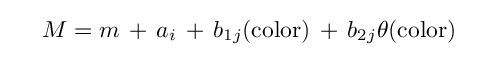
where we now have a constant b1 and a slope b2 term for each chip-plus-detector, and theta is the angle of incidence at which light strikes the detector.
If the sensitivity of each chip is not perfectly uniform across its face, then we need to correct for this "small-scale" flatfielding error. We might approximate the changes in sensitivity as a low-order polynomial function p of (row, col) position on the chip.
Note a significant difference between these simulations and our experiments with real data. The real data consists of measurements made with a single CCD which is centered on the optical axis of its telescope; as a result, the large-scale variations are radially symmetric around the center of the chip. The simulated data, on the other hand, come from detectors scattered all over the SNAP focal plane, all of which are far from the optical axis. We therefore expect asymmetric patterns in sensitivity across each detector.
We have not yet put the color-dependent terms (b1 and b2 in the equations above) into our simulations and analysis.
It is likely that after SNAP has gathered months or years worth of measurements of stars in its ordinary operations, we will want to analyze this much larger collection of relatively faint stars to look for small, uncorrected systematic errors. In that case, it might well be prudent to follow the methods set forth by van der Marel (2003) in order to speed up the computations.
We are testing this general approach to characterizing variations in sensitivity in two ways: by making repeated observations of star fields with a real telescope, and by running artificial data through a simulation of the SNAP telescope. Let us describe briefly our analysis in each case.
We have undertaken an observing program at the WIYN 0.9m telescope to test the stellar flat-field method using the single-chip S2KB imager. We were mainly interested in the remaining error level after the stellar flat correction is applied as well as developing an efficient, repeatable observing technique. Following suggestions from Manfroid, we chose targets among the Stetson Cluster Standards that would sufficiently populate our field of view without too much overlap of stellar sources. For the S2KB, the sparse cluster of NGC2420 fills about 1/3 of the CCD and tracks well over zenith to reduce differential reddening within the field. Our observing cadence pointed the cluster to a 3 by 3 grid covering the entire CCD in a single filter band. In some cases, we took multiple exposures per readount of the CCD to increase our efficiency of observing time.
To pull out the residual spatial differences in photometry across the chip, we first calculate the mean instrumental magnitude of each star with less than 1% Poisson noise. We then calculate the difference of each instrumental magnitude measure of a single star from its mean magnitude as a funciton of position on the CCD. This difference can then be weighted by the poisson noise in a χ2 fit by a spatial correction function to the residuals. The formula is then:
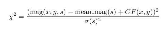
where s is a single star, x and y are the star's coordinates on the chip, and CF is the spatial correction function. As employed by Manfroid and Van der Marel, the correction function is typically a low order 2D polynomial to match any spatial residual while remaining well behaved at the boundaries of the chip. In our tests of S2KB, we found a strong central residual on the chip of about +0.04 magnitudes which could not be well fit by a low order polynomial.
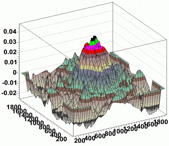
Residuals in photometry (magnitudes) as a function of position
on the detector (pixels) for data taken at WIYN.
Therefore, we used 2-D "Penny2" function (gaussian core with lorentzian wings) which could well fit the central peak, maintain continuity at the chip edges, and keep a low number of fit parameters. We minimize χ2 with this function and determine the fit parameters.
Once the spatial correction function has been calculated, we first applied it to the all of the stars that had less than 0.3% poisson error in their photometry. Since this same stars contributed most heavily to the χ2, this essentially gives us a measure of how well we fit the data. Our results show that the final residual in the fit of our stellar flats is about 0.005 mag RMS. The true test of how well this residual corrects the flatness of photometry across the chip is by applying the correction to another set of stellar measurements dithered over the entire chip. Again using stars with 0.3% statistical photometry error, our final spatially-corrected residual error degrades slightly to 0.006 mag.
We have written a self-contained package for simulating various effects involving variations across the SNAP focal plane. The code is written in a mixture of TCL and C, and is freely available.
This is not a pixel-level simulator; its basic units are stellar measurements. The user provides an input set containing
The program carries out a set of observations, calculating the magnitudes which would be produced in each image from each chip. Although the calculations do not treat individual pixels in each detector, they do include the effects of photon noise, dark current, and other effects on a statistical level.
To illustrate the purpose of this photometric simulator, we show below an example of one set of tests which were made with it.
The input stars in this simulation are based on the USNO-A2.0 catalog of the Northern SNAP field. We point the telescope at RA=270 degrees, Dec=+67 degrees, and then consider only the eastern quadrant of the detector. We include all stars with B and R magnitudes brighter than 18.0, in a one-degree box around the center of the eastern quadrant (RA=271.28, Dec=67.0). That yields about 1840 stars. We assign a spectral type to each star based on its (B-R) color from the USNO-A2.0 catalog. Click on the image below for a larger version.
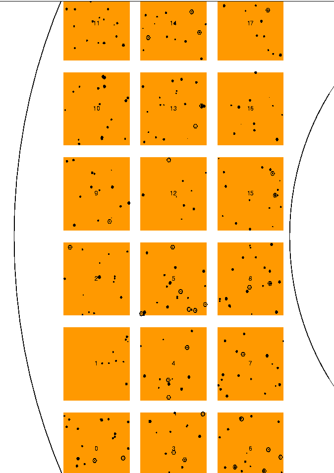
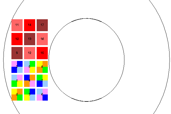
We used both a simplified, "monochromatic" version of the focal plane, in which all detectors were optical CCDs with fiducial filter 5,
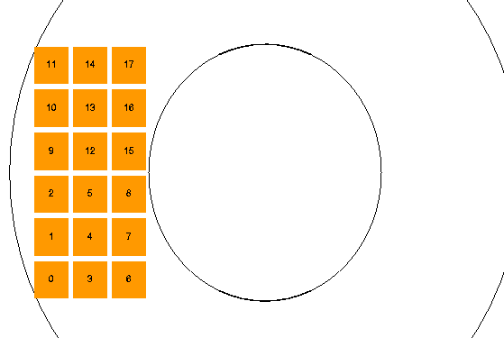
and a realistic focal plane, with a block of optical CCDs and a block of near-IR detectors:
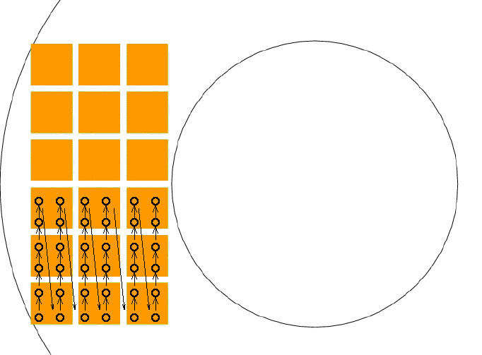
We moved the simulated telescope in a 6x6 grid-like pattern, so that some stars would move across one entire block, appearing at least once on each visible CCD, or at least once on each near-IR detector.
All exposures were 10 seconds long. We used two modes of observing:
Of course, in any particular snapshot, some stars will fall between detectors. Our analysis used Honeycutt's inhomogeneous ensemble photometry technique, including any stars which are detected on at least 10 images.
We did NOT include any of these complicating effects:
The simulator can add all these effects to the "observations", but we are not yet ready to analyze the results in an automated fashion.
In this preliminary simulation, we checked to see how well one can determine the chip-to-chip offsets from a set of exposures which move across a field of stars. We find