Table of Contents
I have written code which simulates measurements of stellar magnitudes by the SNAP telescope. It is not the official SNAP simulation, nor does it have any relationship to the official software. However, it does allow me to calculate the expected signal from a particular sort of star in a given exposure time, and it also permits me to evaluate various schemes for commissioning the telescope when it first reaches orbit.
Since other SNAP calibration team members may find the program useful, I am making it available to all. This document describes briefly how one can download, install, and use the program.
The requirements for running the pipeline are:
Here are very brief instructions for setting things up. I'll follow each step with an example of the procedure.
  % cd /data/
  % mkdir snap
  % cd snap
  %
  % wget http://spiff.rit.edu/richmond/snap/pipeline/aug19_2004/snap_pipeline-0.2.tar.gz
    100%[====================================>] 6,920,628     36.07M/s    ETA 00:00
    13:47:15 (36.07 MB/s) - `snap_pipeline-0.2.tar.gz' saved [6920628/6920628]
  % ls
    snap_pipeline-0.2.tar.gz
  %
  % ls
    snap_pipeline-0.2.tar.gz
  % tar -xzf snap_pipeline-0.2.tar.gz
  % ls
    snap_pipeline-0.2   snap_pipeline-0.2.tar.gz
  %
  % cd snap_pipeline-0.2
  %
  % ./configure
    checking for a BSD-compatible install... /usr/bin/install -c
    checking whether build environment is sane... yes
           (plus lots more like this ...)
    config.status: creating output/Makefile
    config.status: executing depfiles commands
  %
  % make
    Making all in input
    make[1]: Entering directory `/xx/tmp/snap/snap_pipeline-0.2/input'
            (plus lots more like this ....)
    gcc  -g -O2   -o flam_mag  flam_mag.o  -lm
    make[1]: Leaving directory `/xx/tmp/snap/snap_pipeline-0.2'
  %
  % make check
    selftest.pl: running test of SNAP pipeline code ....
    selftest.pl: about to test for tclsh: ..tclsh ./selftest.tcl..
    selftest.pl: about to test for wish: ..wish ./selftest.tcl..
    selftest.pl: going to use wish as interpreter
    selftest.pl: cmd is ..wish ./selftest.tcl >& ./selftest.out..
    selftest.pl: about to run SNAP pipeline; this may take a minute ....
    selftest.pl: you may see a graphics window pop up ....
            (and a window may pop up here ....)
    selftest.pl: all tests passed OK
    PASS: selftest.pl
    ==================
    All 1 tests passed
    ==================
    make[2]: Leaving directory `/xx/tmp/snap/snap_pipeline-0.2'
    make[1]: Leaving directory `/xx/tmp/snap/snap_pipeline-0.2'
  %
If all goes well, you may see a window with a picture of the SNAP focal plane pop up and then disappear after 10 or 20 seconds. The selftest Perl script should end by writing
     PASS: selftest.pl
     ==================
     All 1 tests passed
     ==================
to indicate that the pipeline ran a small test procedure
successfully.
If you now look in the "output" subdirectory,
you ought to see a bunch of files created by the
selftest script.
If the selftest script fails, you can look in the file "selftest.out" for a log of the pipeline's output as it ran. This may give some clue to any errors which occurred. If you need more information, try editing the file snap_driver.tcl to make the "debug" level higher than 2; so, change this:
global debug
set debug 2
to this:
global debug
set debug 6
Then run the "selftest.pl" script again:
% perl selftest.pl
and look once more in the "selftest.out" file
for a more verbose log of the pipeline's operations.
a value of 6 might be
Once the program has been installed, you should have
The file snap_driver.param contains a list of "stages":
# flags to execute (or not) specific pieces of the pipeline
#     1       means execute it
#     0       means skip it
do_setup           1
do_refcat          1
do_focal           1
do_filter          1
do_draw_focal      1
do_telescope       1
do_snapshot        1
By editing this file and changing the values of some of these parameters to 0, one can skip over portions of the pipeline and save time. For example, by running the "refcat" stage once, one will create a catalog of stars which can be used over and over again for many tests; there is no need to re-create the catalog for each one.
One way to run the pipeline is to start a TCL interpreter and then execute commands from the main program:
$ tclsh
% source snap_driver.tcl
For convenience, I've created a small text file, "cmd.in", which contains nothing more than this single source command, so that one can execute the pipeline and capture its output in a single command:
$ tclsh < cmd.in >& cmd.out
The first stage of the pipeline simply modifies the parameter files so that they indicate the proper values for the current installation. The file setup.param is an ASCII text file; part of it looks like this:
# directory containing the input data: focal plane info, filter
#     transmission curves, star catalogs, etc.
input_dir       ./input
The input_dir parameter is defined here to have the value "./input", meaning that input files can be found in a subdirectory of the current directory called "input". Many other parameter files contain this same variable input_dir.
If you wanted to move the installation so that all the input files were located somewhere else, you might edit the file so that read
# directory containing the input data: focal plane info, filter
#     transmission curves, star catalogs, etc.
input_dir       /home/fred/snap/input
Since input_dir appears in other parameter files, you could edit all of them, too, making the same change in each. However, there is an easier way: when the "setup" stage runs, it takes the values of any parameters in the setup.param file and copies their values to all the other parameter files. By changing just one file, setup.param, and then running the "setup" stage of the pipeline, any changes are disseminated to all relevant files.
The second stage of the pipeline prepares the overall transmission curves we will use for each detector on the focal plane. In the input_dir are the components which affect the spectral efficiency of the instrument:
The "filter" stage of the pipeline convolves these factors in the appropriate way to generate overall transmission curves as a function of wavelength. It places into the output_dir two things:
    filt_000 {   0  000A   0   1   5   1 filt_000A.dat }
    filt_001 {   1  000B   0   2   3   1 filt_000B.dat }
    filt_002 {   2  000C   0   3   4   1 filt_000C.dat }
The zero'th filter lies on quadrant "A" of the
chip with index 0. It is based on the fiducial filter
with index 5 (the reddest visible filter),
but its overall transmission can be found in the
file "filt_000A.dat" in the output_dir.
      8407.0000     0.6792
      8408.0000     0.6800
      8409.0000     0.6809
in which the first column is the wavelength in Angstroms,
and the second column the throughput at that wavelength,
on a scale of 0.0 - 1.0.
This stage of the pipeline uses the executable program spec_convolve to combine all the individual transmission curves into a single overall curve.
The user must supply a set of stars which will be run through the telescope and detectors. This stage of the pipeline converts the input catalog from a format which is relatively easy to provide into one which the code can use.
The input format is based on that of the USNO A2.0 catalog, as provided by SIMBAD's Vizier query facilty. If one visits Vizier and queries this catalog around the position RA=18:00:00 and Dec=+67:00:00, with a search radius of 5 arcminutes, requesting output position in decimal degrees, one will receive a list like so:
#Full    _r      _RAJ2000      _DEJ2000    USNO-A2.0       RA(ICRS)    DE(ICRS)  ACTflag Mflag  Bmag  Rmag    Epoch
#      arcmin     "h:m:s"       "d:m:s"                       deg         deg                    mag   mag     yr
    1  0.4936  269.999675   67.008225  1500-06401275  269.999675   67.008225                18.3  17.8  1952.631
    2  0.7868  270.013567   67.011995  1500-06401517  270.013567   67.011995                18.5  18.5  1952.631
    3  0.8811  270.030500   67.008584  1500-06401783  270.030500   67.008584                14.3  13.4  1952.631
    4  0.9718  270.024300   66.986881  1500-06401699  270.024300   66.986881                16.6  16.2  1952.631
    5  1.0931  269.957114   66.992856  1500-06400616  269.957114   66.992856                18.7  18.5  1952.631
Note that this list includes position (J2000), the B-band magnitude and R-band magnitude. These are (almost) the only pieces used by the pipeline. It uses the (B-R) color to look up and interpolate the spectral type of a star in the file input_dir/calc_colors.out. A guess at the V-band magnitude is determined by taking the average of the B and R magnitudes. Using a set of template spectra from Pickles , the pipeline generates synthetic magnitudes for the star in all nine fiducial SNAP passbands. It writes into the output_dir a catalog containing the same stars in a somewhat different format, like this:
 269.99968   67.00822     f5v  29.278   1 18.050    0 18.309   2 17.931   3 17.8 87   4 17.877   5 17.896   6 17.949   7 18.046   8 18.179
 270.01357   67.01199     a5v  29.819   1 18.500    0 18.544   2 18.554   3 18.6 56   4 18.737   5 18.807   6 18.906   7 19.116   8 19.378
 270.03050   67.00858     k0v  24.973   1 13.850    0 14.339   2 13.553   3 13.3 46   4 13.233   5 13.180   6 13.174   7 13.213   8 13.245
 270.02430   66.98688     f5v  27.628   1 16.400    0 16.659   2 16.281   3 16.2 37   4 16.227   5 16.246   6 16.299   7 16.396   8 16.529
There first element in the list of (filter index, magnitude) has an index of 1; the pipeline assumes that the fiducial SNAP passband number 1 (a slightly redshifted B-band) is close to the Johnson-Cousins V-band, and uses it to normalize magnitudes of stars of different spectral types. That is, it forces an O-star of magnitude V=20 to have the same number of photons in SNAP passband 1 as an M-star of magnitude V=20.
What about light from the sky background? If the user wishes calculations to include the background, he must place into the input catalog of stars a special entry for the sky; my calculations of the background sky brightness indicate that an entry should look like:
9999 sky 271.271281 66.744063 QQ 271.671281 66.744063 23.52 23.52 0.000The RA and Dec, elements 3 and 4, can be modified as desired; it is the magnitude values near the end of this line which are important.
This has special features:
If the input catalog does not contain any "sky" entry, then the calculations of signal and noise will use a sky value of zero.
This stage of the pipeline does very little. It calculates the effective collecting area of the telescope. It also sets the factor by which the telescope optics illuminate one portion of the focal plane differently than another; by default, there is no variation in illumination.
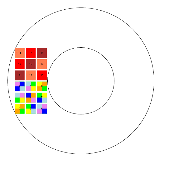
The SNAP focal plane is a complicated structure: it contains 72 detectors arranged in four quadrants around an annulus. Some of the detectors (the IR ones) have a single filter covering their entire surface, but others (the visible CCDs) are split into four pieces with a different filter in front of each. Moreover, the detectors in each quadrant are rotated relative to each other.
This stage goes through the tedious process of figuring out exactly where on the focal plane each detector lies, how it is rotated, which filters lie in front of it, and so forth. It writes a file into the current directory (not the output_dir) indicated by the foc_output_file parameter in focal.param, which contains a list of all the chips and their properties. This file is then used by other code further downstream.
Note that the parameter file focal.param for this stage contains a great deal of information on the layout of the focal plane and properties of the detectors. For example, the lines
# default properties of visible CCD detectors
foc_vis_prop { { dark 0.0005 } { read 4  } { gain 2.0 } { sat 130000 } { offset 0.0 } }
# default properties of the IR detectors
foc_ir_prop  { { dark 0.04   } { read 20 } { gain 2.0 } { sat 100000 } { offset 0.0 } }
describe the readout noise, dark current, saturation levels, etc., for the visible and near-IR detectors.
The user can control the cosmetic quality of the detectors via the foc_chip_variation parameter. Possible values are
- none
- each detector has uniform response across its area
- center
- each detector has an identical radial decrease in sensitivity away from its center
- linear
- each detector has an identical linear decrease in sensitivity in one direction, uniform response in the other
- random
- each detector has a different random decrease in sensitivity in an elliptical pattern around a random location on the chip
Any variations are described by a simple polynomial of the form
                                             1.0
   relative sensitivity  =  -------------------------------------
                            a + b*x + c*y + d*x*x + e*x*y + f*y*y
where x = (row - row0), y = (col - col0),
and (row0, col0) is the location with peak sensitivity.
The numerical coefficients of the polynomials describing
the variations (if any) will be written into the file
indicated by the foc_output_file parameter.
The parameter foc_east_only in focal.param controls whether the detectors are in the East quadrant only (set foc_east_only to 1)
or fill the entire focal plane (set foc_east_only to 0)
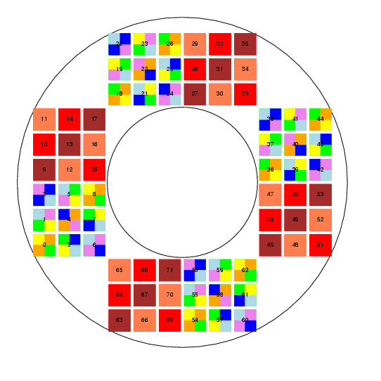
If the user chooses to execute the draw_focal stage, and if the graphical Tk interpreter is available, then the code will draw a Postscript picture of the focal plane and place it in the output_dir. The name of the output file is set by the output_file parameter in focal.param.
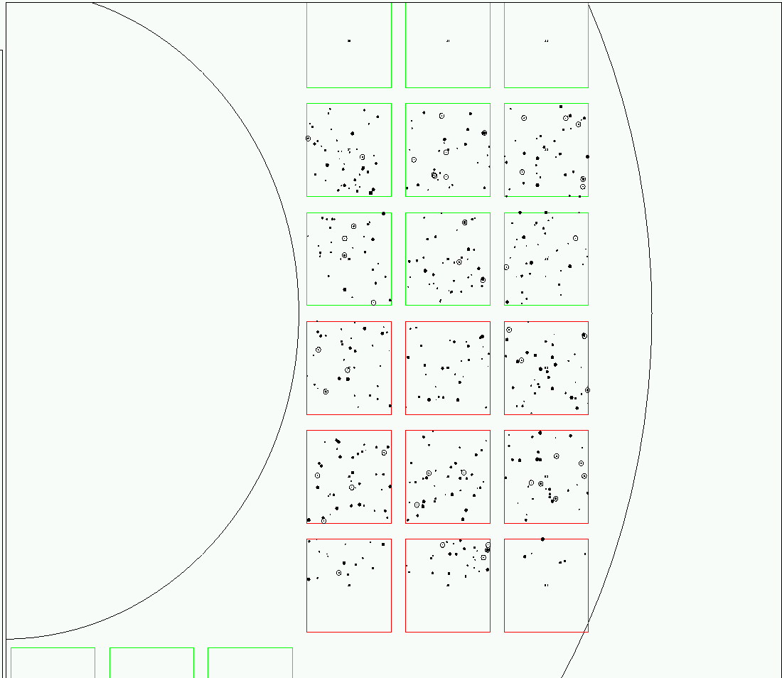
If the user goes on to take a snapshot, then this picture will have placed on it a depiction of all detected stars. As described in my status report of August 21, 2003, the picture uses dots and circles of different sizes to indicate stars of different magnitudes:
The heart of the pipeline is the calculation of the instrumental magnitude of each star which falls on a detector. Variables in snapshot.param allow the user to take one or many "snapshots": each snapshot is a single simultaneous exposure of all the detectors. The parameters
snapshot_step_ra            0.0
snapshot_step_dec          -0.01
describe how far (in degrees) the telescope moves from one snapshot to the next. At the moment, the user can specify only a single pass of linear motion.
The calculations follow this path:
In order to determine the uncertainty in the measurement, we follow the simple model of Howell (1989)
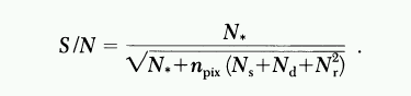
We use synthetic aperture photometry, with a circular aperture of size given by the snapshot_aper_rad parameter, and assume all the starlight falls within the aperture. We calculate the signal-to-noise ratio for the measurement, and turn that into an uncertainty in magnitude using
                                   1.0
          mag_uncertainty  =  ---------------
                              signal_to_noise
If the parameter snapshot_add_noise in the snapshot.param file is set to 1, then a random value drawn from a gaussian distribution with standard deviation equal to this uncertainty is added to the magnitude measurement. If the snapshot_add_noise parameter is zero, then the magnitude is left in its "perfect" state.
The measurements are placed into the output_dir in two different files (or sets of files).
        271.27128  66.74406  22.9827  0.0658
        271.55585  66.85864  19.4291  0.0079
        271.55585  66.85864  19.9742  0.0104
 271.27128  66.74406     sky 34.659  23.908 23.520 23.269 23.079 22.971 23.070 23.316 23.464 23.571     3 2054.01  574.22  -191.09  -95.49   213.62 0.22324  23.520  12   1  22.983  0.066  -0.537
 271.55585  66.85864     a0v 31.385  19.955 20.000 20.133 20.292 20.431 20.560 20.715 20.945 21.198     1 2195.03  438.93  -232.77  -50.91   238.27 0.24606  19.955   4   0  19.429  0.008  -0.526
 271.55585  66.85864     g0v 31.197  20.346 20.000 19.824 19.707 19.633 19.627 19.679 19.783 19.893     1 2195.03  438.93  -232.77  -50.91   238.27 0.24606  20.346   4   0  19.974  0.010  -0.372
The "verbose" output files allow one to search for variations in observed magnitude as a function of position in focal plane, or stellar color, etc. The fields in the verbose output are
The instrumental magnitudes produced by the pipeline have the form
mag = mag_zero - 2.5*log10( num_photons )
where the value of "mag_zero" is given by the snapshot_mag_zero
parameter in the snapshot.param file;
its default value is 30.0.
So, for example, if the given star appears in an output file with
magnitude 24.65, then the number of detected photons must be
                               0.4*(mag_zero - mag)
            num_photons  =  10

                               0.4*(30 - 24.65)
                         =  10                    =   138
Yes, but it will take a bit of work. The input directory contains a set of files containing the default passbands for the SNAP filters, with names like fiducial_b0.filter, fiducial_b1.filter, etc. You may either modify by hand the values in these files, or create a different set of files with the same simple 2-column ASCII format; then re-run the do_filter step of the pipeline. This should create a new set of overall (filter plus mirrors plus detectors) passband files in the output directory with names like filt_003A.dat.