During the first few weeks and months of the SNAP mission, the spacecraft will perform special calibration tasks. One of these tasks will involve cross-checking each of the detectors on the focal plane against others of its kind (e.g., all visible CCDs with filter 2 against each other, all IR detectors with filter 7 against each other). There are several parameters one can imagine using to control these cross-calibration tasks:
This is clearly a large parameter space. I am starting to use my simple photometric pipeline to study the commissioning phase. In this early (and non-definitive) document, I consider issues 1-4 in the list above.
One of the basic ideas is that the spacecraft will slew gradually across some portion of the sky, causing stars to move from one detector on the focal plane to another to another.
By comparing the instrumental magnitudes of one group of stars as they move from detector "A" to detector "B", we can easily determine any fixed offset between the two detectors; with somewhat more effort, we can check for systematic differences in color terms, intra-chip flatfield variations, and other subtle effects.
For simplicity's sake, I used stars of spectral type A0V only in the tests described below; I also chose to use SNAP filter 6 (the bluest of the IR bandpasses) only. I will run similar tests with a more exhaustive set of input parameters later.
Exposure times
Using numbers from Some stellar statistics in the SNAP field , I find that the number of stars falling on each detector will be roughly
----------------------------------------------------
 V magnitude      14      15      16      17
 stars/chip       1.2     2.5     3.5     5.0
----------------------------------------------------
Clearly, a network of stars used for calibration must be at least sixteenth or seventeenth magnitude, or fainter, in order to provide more than one star per chip in each image. The fainter the stars in this network, however, the longer all exposure times must be to build up decent signal-to-noise. For the purposes of these tests, I chose stars between magnitude V=16.0 and V=17.0, which I will call "sixteenth magnitude" from here on.
Using the pipeline, I simulated a number of images of the same set of stars and looked at the scatter in the resulting mean instrumental magnitude of each star.
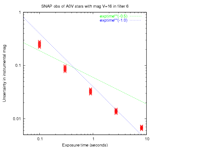
The scatter drops with exposure time, of course. For very short exposure times, the scatter drops almost as the reciprocal of the exposure time (i.e. exposure twice as long, cut the uncertainty in half). At these shortest exposure times, the readnoise dominates the noise; since it is fixed -- it doesn't change with exposure time -- the noise is roughly constant. As we increase exposure time, we increase the signal with very little increase in noise; thus, an inverse linear relationship.
For exposure times longer than about 10 seconds, however, the variance in the number of photons from the star itself start to dominate the overall noise. That means that the signal-to-noise ratio increases only as the square root of the exposure time.
Note that for this combination of stellar type and bandpass, the scatter in individual magnitude measurements drops below 1 percent (0.01 mag) at an exposure time of 5 to 10 seconds. I will use the longest exposure time in my tests (8.1 seconds) in most of the plots shown below.
I will now run through the results of a number of tests, in which I varied one parameter and looked at the resulting changes (if any) in the determination of the offset between chip A and chip B as a group of stars moved from one to the other. In this simulation, the true offset between the chips was zero; in other words, the two detectors were assumed to be identical.
In each test, I generated images of a group of stars, (the group size ranging from 4 to 32 stars), sometimes repeating exposures at a given position, as the group migrated from one detector to another. I then ran the instrumental magnitudes through software based on Kent Honeycutt's article on inhomogeneous ensemble photometry to derive both the (relative) magnitude of each star and the offset between the chips. I did not include effects due to shifts in filter passbands with incidence angle, intra-chip variations in sensitivity, and other high-order complications (though the pipeline is able to produce them).
I did add random gaussian noise, based on the signal-to-noise ratio for each star, to its instrumental magnitude. I generated 5 realizations of each image, ran them all through the analysis package, and then calculated the mean and standard deviation from the mean for the chip-to-chip offset. I can see now that I should have used a larger number of realizations -- perhaps 25 or 30.
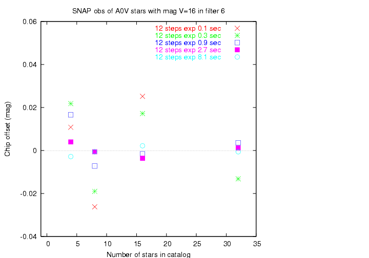
As a simple test of this framework, we would expect that the offset can be determined more precisely with longer exposure times, since the measurement of each star will be more accurate. Let's see ...
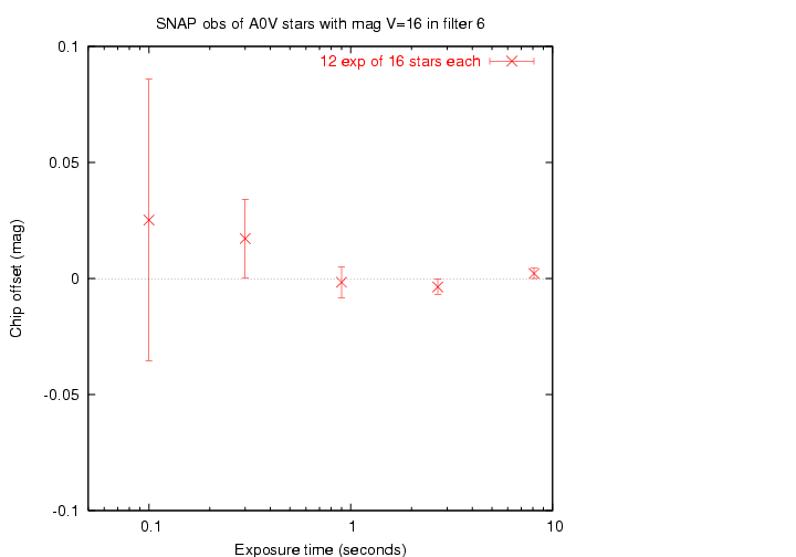
Yes, we get closer to the true offset (zero) with longer exposure times. Good.
We saw above how the uncertainty in the measurement of a single star decreases with exposure time: roughly as 1/t for short exposure times t, and as 1/sqrt(t) for longer exposures. Does the uncertainty in the determination of chip-to-chip offset follow the same pattern?
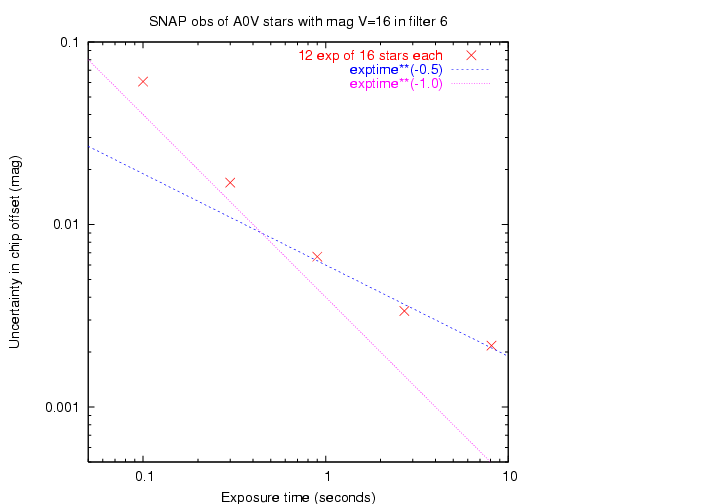
Reasonably so. Good.
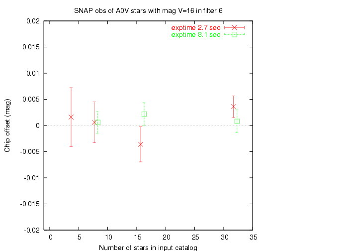
It would seem logical that the larger the number of stars in the input set, the better we can determine the offset between chips.
Hmmm. I draw two conclusions:
A few very precise measurements would appear to be nearly as good for our purposes as many less precise ones. However, this is one test I wish to revisit with more random realizations.
Which is a better way to spend one hour of time on orbit during the commissioning phase?
In other words, if we end up with the same number of instrumental magnitudes (with the same signal-to-noise ratio), does it matter if they come from repeated measurements of a small set of stars, or from a few measurements of a larger set?
I ran tests in which I measured 192 instrumental magnitudes during a gradual motion from chip A to chip B. In some tests, there were only 4 stars in the sky, so I repeated many exposures at each position; in others, there were up to 32 stars in the sky, so I made fewer repeated images at each step. Below, I show the results for images with two different exposure times (both of which yield good signal-to-noise in each magnitude).
I see a weak improvement as the number of unique stars grows.
At each pointing of the telescope, we can take a single image and then slew again, or we can take a series of exposures. For other reasons (cosmic rays) beyond the scope of my simulation, it makes sense to take multiple exposures at each position. However, I thought I'd see what effect it had on the chip-to-chip offset in this very simple model.
I created an input catalog of only 4 stars, arranged so that they gradually moved from one chip to the other over a series of 3 steps in pointing. At each step, I took 1, 2, 4, 8, or 16 exposures.
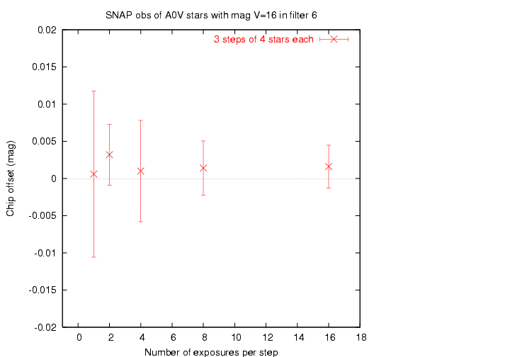
Yes, repeated exposures do help ... but the rate of improvement slows down rapidly. This suggests to me that we should take the 3 or 4 exposures at each position required to remove cosmic rays, but no more than that.
Suppose one is going to take 12 exposures as a group of stars moves from chip A to chip B. One could take
In other words, one can distribute the motion into a few large steps, or many small steps. Does it make a difference?
For reasons I did NOT consider in this simulation -- variations in sensitivity across a single detector, aka "single-chip flatfield" -- it is important to make many small steps.
I ran several tests in which the total number of measurements was the same (either 48 or 96 instrumental magnitudes), but they were distributed into several big steps with many repeated exposures, or many small steps with few repeated exposures. Look for variation within symbols of the same color in the graph below.
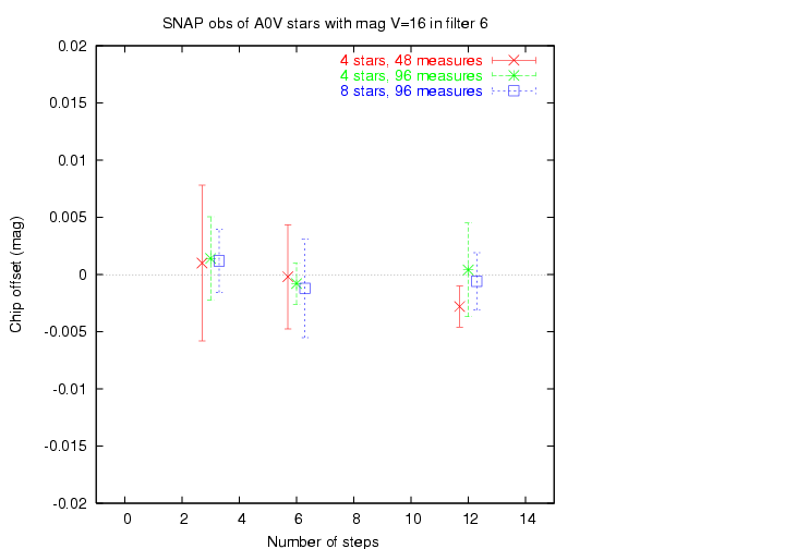
There is little apparent difference in these two approaches; therefore, it is reasonable to use many small steps, for the reasons mentioned paranthetically above.