Tomoe Note 022: Search for transients in "FAST Survey" data of 20201217

Michael Richmond
Jan 8, 2021

Executive Summary

On Dec 17, 2020, the Tomo-e camera carried out a relatively short (approx 1 hour) survey of regions cooperatively with the FAST telescope, looking for fast radio bursts. Only 1/3 of the chips were used to collect data (as far as I can tell). My search revealed no transients with durations of 3-20 seconds.

The dataset for 20201217

The dataset "20201217" is based on images acquired during UT 2019 Dec 17, with PROJECT name 'FAST survey' and OBSERVER 'Y. Niino'. The images cover the span of time



    2459201.298  ≤   JD  ≤ 2459201.375

with a gap in the middle. The span of active collection time is only about 60 minutes, and much of the second half of that time is plagued by clouds. All four quadrants were active, but data from only 1/3 of all the chips was saved, as far as I can tell. This is therefore a small datatset.

The FITS headers of one of these images states, in part:

OBJECT  = 'FASTsurvey'         / object name                                    
EXPTIME =            59.994240 / [s] total exposure time                        
TELAPSE =            60.500020 / [s] elapsed time                               
EXPTIME1=             0.999904 / [s] exposure time per frame                    
TFRAME  =             1.000000 / [s] frame interval in seconds                  
DATA-FPS=             1.000000 / [Hz] frame per second                          
DATA-TYP= 'OBJECT'             / data type (OBJECT,FLAT,DARK)                   
OBS-MOD = 'Imaging'            / observation mode                               
FILTER  = 'BLANK'              / filter name                                    
PROJECT = 'FAST survey'        / project name                                   
OBSERVER= 'Y. Niino'           / observer name                                  
PIPELINE= 'wcs,neo,stack,raw'  / reduction pipeline templete

The images were reduced and cleaned by others; I started with clean versions of the images. Each set of 60 images was packed into a single FITS file, covering a span of (60 * 1.0 sec) = 60 seconds. These "chunk" files were transferred to shinohara by me, and placed in

   /gwkiso/tomoesn/richmond/work/work_20201217

with names like

   rTMQ2202012170043926213.fits

These names can be decoded as follows:


       r             stands for    "reduced" ??
       TMQ2          means         "Tomoe data, part of quadrant 2"
       20201217      means         year 2020, month 12, day 17
       00439262      means         chunk index 00439262 (increased with time)
       13            means         chip 13
       .fits         means         a FITS file

I'll refer to each of these "composite" files as a "chunk".

There are typically 43 chunks for each chip, and a total of 1358 chunks in the entire dataset. Each chunk file was 541 MByte, so the total volume of the chunk files was about 734 GByte = 0.7 TByte.

Brief description of the pipeline analysis

I ran a slightly modified version of the Tomoe pipeline on the images; it was not the same as that used to analyze the 2016 images discussed in the transient paper for two reasons:

minor modifications to handle the slightly different format of the data (image size and overscan regions)
small improvements in the astrometric procedures to make the routines more robust

The main stages in the pipeline were:

split a chunk into individual images (60 images per chunk)
detect and measure stars in each image
add the Julian Date to each stellar measurement
perform ensemble photometry of all images in the chunk
perform astrometric and photometric calibration of the stars included in the ensemble (some stars, detected in only a small number of images, will not be included in the ensemble)
perform astrometric and photometric calibration of all stars detected in each image individually

The output of the pipeline includes a copy of each FITS image, plus a set of ASCII text files which include both the raw, uncalibrated star lists, and the calibrated versions of those lists, as well as the ensemble output. Let's compare the sizes of the input and output for quadrant 1:

input: 687 GByte
output: 346 GByte (including FITS images), 7 GByte (ASCII files only)

Note that the input images contain 32 bits per pixel, while the output images created by the pipeline have only 16 bits per pixel. Thus, the output images are only half the size of the input. Aside from the FITS images, all the other text output of the pipeline is very small.

Location on the sky

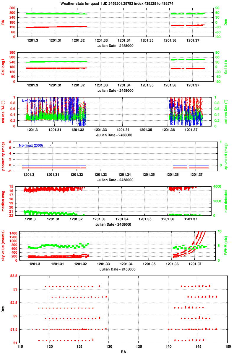
The figure below shows, in the bottom panel, the (RA, Dec) location of these observations. The fields are relatively far from the plane of the Milky Way, at galactic latitude 30-45 degrees (as shown in the second panel).

"Weather" plots for the 4 quadrants

After running the pipeline to reduce the data, clean the images, find and measure stars, calibrate them astrometrically and photometrically, I used a script to look at properties of the data over the course of the night. You can read more about the "weather" in another note.

Below are links to the graphs produced for each of the 4 quadrants.

Quadrant 1:

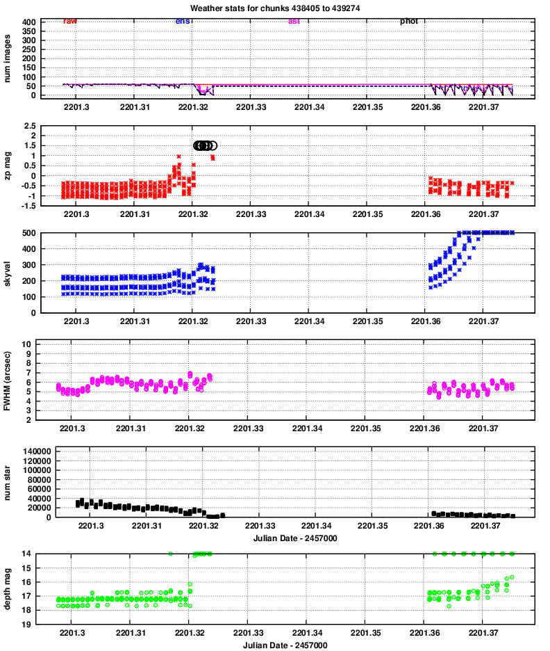
Quadrant 2:

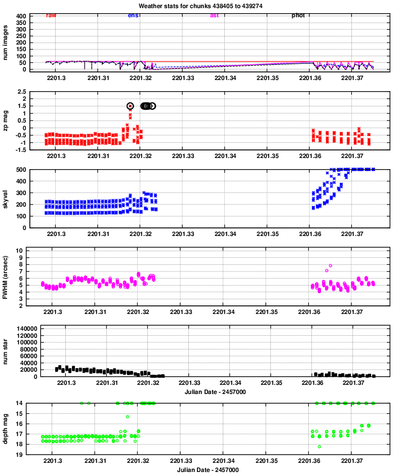
Quadrant 3:

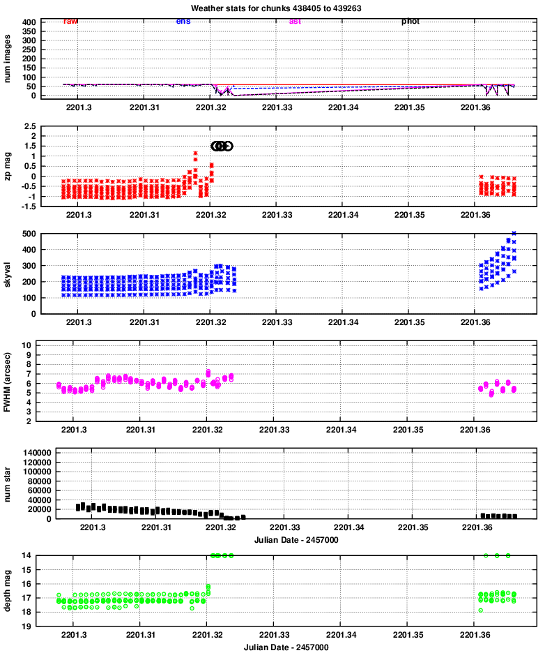
Quadrant 4:

What do we learn from the "weather" graphs?

zp mag: the "zero-point" shown here is related to the difference between the instrumental magnitudes of stars in each image, and the calibrated magnitudes of those stars:
```
               zp  = (instrumental_mag) - (calibrated_mag)

     
```
Large positive values indicate extinction due to the atmosphere or clouds.
Near the end of the first set of images, the zero-point rose -- that's due to clouds. I guess that clouds stopped the observations for a while, explaining the gap.

sky value: this is simply the typical number of counts per pixel in the photometric annulus around stars. This shows a small increase before the gap, and a large increase at the very end: that was probably dawn.

FWHM: the typical Full-Width at Half-Maximum for stars in each image, converted from pixels to arcseconds. We see values of 5-6 arcseconds.

number of stars: this is the total number of detections of stars in all the images for a given chip, during each chunk. In other words, if one bright star appears in all the 120 images of that chunk, it will contribute 120 units toward this total.
There is a drop in the number of stars detected with time, probably due to clouds, then the rising brightness due to dawn.

depth mag: this is not the same thing as the "limiting magnitude" assigned to each chunk; it is a slightly different quantity which does give the same sense of "how faint are the stars typically detected in this chunk?" The method by which it is calculated is pretty simple:
- place all detected stars into bins by magnitude
- pick the bin with the largest number of stars
- compute the median magnitude in that bin
The images typically show stars down to mag V = 17 and a bit fainter, which is relatively normal.

Transients and control time

After all the data had been calibrated, I ran the "transient_a.pl" script, which applies the rules described in the Tomo-e transient search paper to look for sources with only a brief existence. The code also computes a "control time" for the dataset.

The software found 343, 333, 242, 285 candidates in quadrants 1, 2, 3, and 4, respectively. This is roughly 10 times as many as were found in the Nov-Dec 2019 dataset. I created a web page showing the properties of these candidates in each quadrant:

The entry for each candidate includes some information about the chunk in which it appears, its position in (x,y) pixel coordinates and (RA, Dec) coordinates, and its magnitude. The "variability score" describes the ratio of the standard deviation of its magnitudes away from the mean to the standard deviation from the mean of stars of similar brightness; so, a high score means the object is varying from frame to frame more than most objects of similar brightness.

The entries also contain columns listing the magnitudes of any objects at this position (to within 5 arcsec) in the USNO B1.0 (avergage of R-band magnitudes) and in the 2MASS catalog (K-band magnitude). A value of "99.0" indicates that no source appears in the catalog as this position. You can see that the overwhelming majority of candidates do correspond to objects which were detected in one or both of these catalogs -- meaning that they are not true transients.

After these columns of text, the documents contain thumbnails of the images around the candidate. The thumbnails are oriented with North up, East left, and are 110 pixels (= 130 arcsec) on a side.

I found no candidates which looked like real transients in this dataset; feel free to examine them yourself.

The table below shows the control times for each quadrant in this dataset:


quadrant         control time (square degrees * sec)
                   V=13     V=14     V=15     V=16  
--------------------------------------------------------
  1                3896     3762     3123      224
  2                3060     2991     2753      581
  3                3445     3378     3036      134
  4                3450     3285     2582       27 

 total            13851    13416    11764      966
--------------------------------------------------------

The total control time is of order 1,000 square degrees times seconds, down to a limit of V=16 in a 1-second exposure.

These control times are much smaller than the control times listed in the transient paper.