I have analyzed a dataset involving all 84 chips. The run covers just over one hour (62 minutes). Conditions were good, but no promising transient candidates were found.
The dataset "20191123" is based on images acquired during UT 2019 Nov 23. The images cover the span of time
2458811.1065920 ≤ JD ≤ 2458811.1494690
which is about 62 minutes.
The FITS headers of one of these images states, in part:
OBJECT  = 'J0350+1735_dith1'   / object name
EXPTIME =           119.988480 / [s] total exposure time
TELAPSE =           120.500020 / [s] elapsed time
EXPTIME1=             0.999904 / [s] exposure time per frame
TFRAME  =             1.000000 / [s] frame interval in seconds
DATA-FPS=             1.000000 / [Hz] frame per second
DATA-TYP= 'OBJECT'             / data type (OBJECT,FLAT,DARK)
OBS-MOD = 'Imaging'            / observation mode
FILTER  = 'BLANK'              / filter name
PROJECT = 'Earth Shadow 2Hz Survey' / project name
OBSERVER= 'Noriaki Arima'      / observer name
PIPELINE= 'wcs,stack,raw'      / reduction pipeline templete
Note that the exposure time is 1.0 seconds per frame, which is not the same as the 0.5 seconds per frame for earlier nights in this series of data. Yes, the "PROJECT" name says "2Hz", but this is really 1 Hz.
The images were reduced and cleaned by others; I started with clean versions of the images. Each set of 120 images was packed into a single FITS file, covering a span of (120 * 1.0 sec) = 120 seconds. These "chunk" files were located on shinohara in the directory
/gwkiso/tomoesn/raw/20191123
with names like
rTMQ2201911230018485632.fits
These names can be decoded as follows:
       r             stands for    "reduced" ??
       TMQ2          means         "Tomoe data, part of quadrant 2"
       20191123      means         year 2019, month 11, day 23
       00184856      means         chunk index 00184856 (increases with time)
       32            means         chip 32
       .fits         means         a FITS file
I'll refer to each of these "composite" files as a "chunk".
There are typically 120 chunks for each chip, and a total of 2490 chunks in the entire dataset. Each chunk file was 1083 MByte, so the total volume of the chunk files was about 2700 GByte = 2.7 TByte.
I ran a slightly modified version of the Tomoe pipeline on the images; it was not the same as that used to analyze the 2016 images discussed in the transient paper for two reasons:
The main stages in the pipeline were:
The output of the pipeline includes a copy of each FITS image, plus a set of ASCII text files which include both the raw, uncalibrated star lists, and the calibrated versions of those lists, as well as the ensemble output.
On the machine shinohara1.kiso.ioa.s.u-tokyo.ac.jp, I ran the pipeline using a single thread; in other words, each chunk, and each image, was sent through the calculations sequentially. There was no attempt at parallel processing.
I ran the main script on each of the four quadrants simultaneously. That is, I started one process in the background, then started a second, then a third, then a fourth. The time taken to process each quadrant was:
  quad      number of chunks     elased time (min)     minutes/chunk
----------------------------------------------------------------------
   1             630               1308                    2.08
   2             630               1442                    2.29

   3             600               1189                    1.98
   4             630               1208                    1.92
----------------------------------------------------------------------
These times are a bit slower than the time to process a chunk when only one quadrant is analyzed at a time: about 1.3-1.4 minutes per chunk. However, running several quadrants simultaneously does result in somewhat faster analysis. Using results from my calculations on nights 20191120, 20191121, and 20191123, I find roughly
   number of quadrants processed      minutes           normalized
      simultaneously                 per chunk       minutes per chunk
------------------------------------------------------------------------
            1                       1.30, 1.46             1.4

            3                       1.91, 1.82, 1.78       0.61

            4                 1.92, 2.08, 2.29, 1.98       0.52
------------------------------------------------------------------------
Running 4 pipelines simultaneously does NOT produce results 4 times faster; instead, it produces results about 2 times faster. I suspect that running more pipelines simultaneously on shinohara would yield dimishing returns; my guess is that disk I/O is becoming the limiting factor.
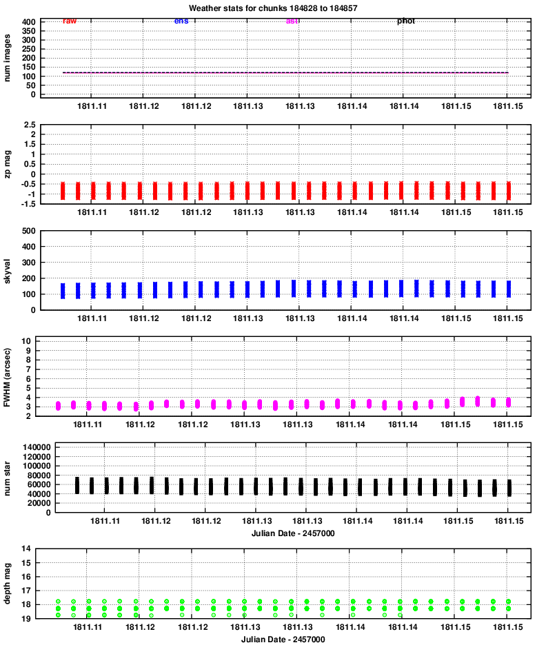
After running the pipeline to reduce the data, clean the images, find and measure stars, calibrate them astrometrically and photometrically, I used a script to look at properties of the data over the course of the night. You can read more about the "weather" in another note.
Below are links to the graphs produced for each of the 4 quadrants.
Quadrant 1:
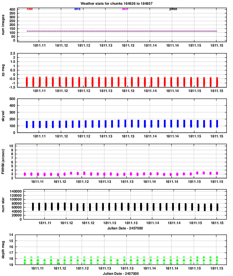
Quadrant 2:
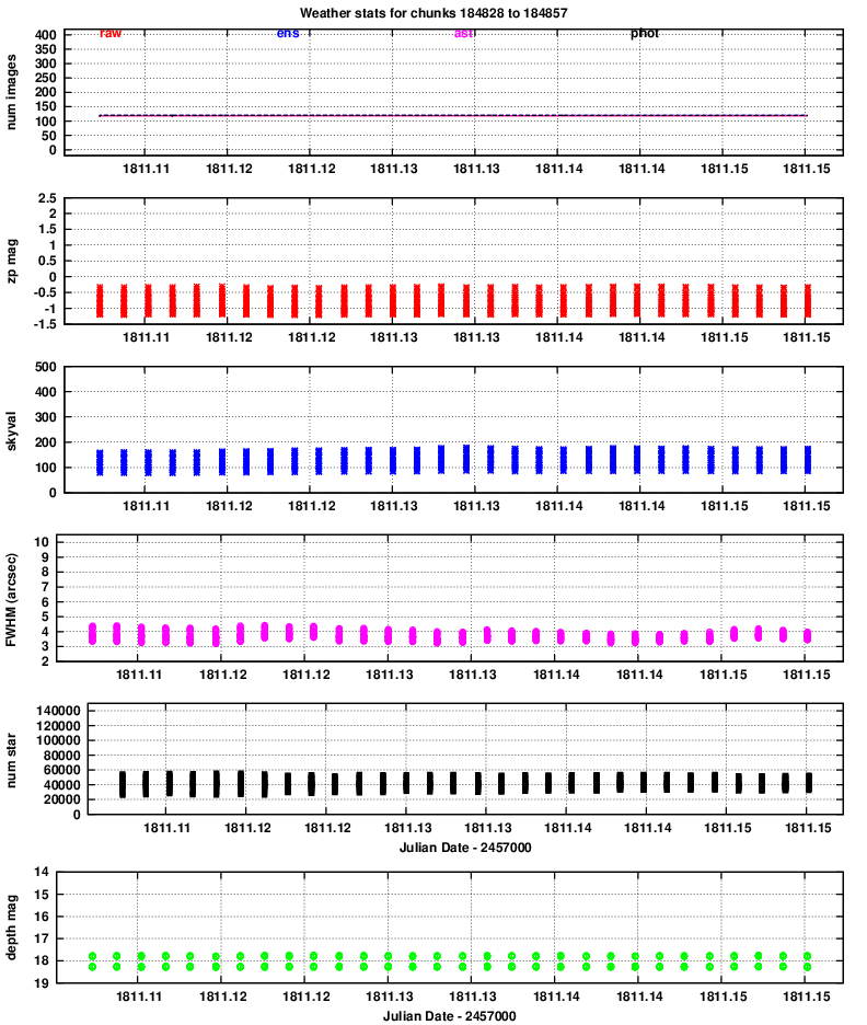
Quadrant 3:
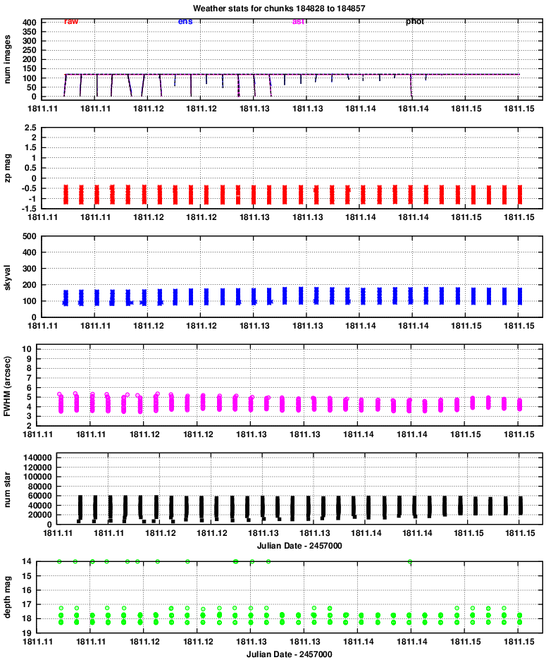
Quadrant 4:
zp = (instrumental_mag) - (calibrated_mag)
Large positive values indicate extinction due to the atmosphere or clouds.
Very small changes means "no clouds tonight."
It is clear that the FWHM for quadrants 3 and especially 4 is (again) considerably larger than that of quadrants 1 and 2.
The images typically show stars down to below mag V = 18, which is the best performance I've seen so far. Of course, the exposure time was increased from 0.5 to 1.0 seconds for this night, so it's not surprising that fainter stars can be detected. We can see that, again, quadrants 3 and especially 4 have slightly lower quality than quadrants 1 and 2.
These patterns are the same as seen in night 20191120 and 20191121.
After all the data had been calibrated, I ran the "transient_a.pl" script, which applies the rules described in the Tomo-e transient search paper to look for sources with only a brief existence. The code also computes a "control time" for the dataset.
The software found 41, 49, 53, and 30 candidates in quadrants 1, 2, 3, and 4, respectively. I created a web page showing the properties of these candidates in each quadrant:
The entry for each candidate includes some information about the chunk in which it appears, its position in (x,y) pixel coordinates and (RA, Dec) coordinates, and its magnitude. The "variability score" describes the ratio of the standard deviation of its magnitudes away from the mean to the standard deviation from the mean of stars of similar brightness; so, a high score means the object is varying from frame to frame more than most objects of similar brightness.
The entries for quadrants 2, 3, and 4, contain columns listing the magnitudes of any objects at this position (to within 5 arcsec) in the USNO B1.0 (avergage of R-band magnitudes) and in the 2MASS catalog (K-band magnitude). A value of "99.0" indicates that no source appears in the catalog as this position. You can see that the overwhelming majority of candidates do correspond to objects which were detected in one or both of these catalogs -- meaning that they are not true transients.
After these columns of text, the documents contain thumbnails of the images around the candidate. The thumbnails are oriented with North up, East left, and are 110 pixels (= 130 arcsec) on a side.
None of these candidates was promising. Roughly 15-20% of the candidates were spurious junk in the wings of a bright star; the rest were mostly very faint stars that appeared briefly above the noise threshold.
The table below shows the control times for each quadrant in this dataset:
quadrant         control time (square degrees * sec)
                   V=13     V=14     V=15     V=16    V=17
-------------------------------------------------------------
  1               18122    18122    18122    18122    6040
  2               18122    18122    18122    18122   10758
  3               17256    17256    17256    17256     747
  4               17220    17220    17220    16920      86

 total            70720    70720    70720    70420   17631
-------------------------------------------------------------
These control times are larger than those for each of the nights listed in the transient paper;