small fixes to control times 5/30/2020
I have analyzed a dataset from the complete camera = 84 chips, but covering less than one hour of a single night. With only small modifications, the same pipeline used for the analysis of 8 nights in 2016 produces good results for all 84 chips. No promising transient candidates were found.
The dataset "20191120" is based on images acquired during UT 2019 Nov 20. The images cover the span of time
2458808.10677 ≤ JD ≤ 2458808.13508
which is only about 41 minutes; so, this is a very short period of time, much less than a full night. However, the dataset includes images from all 4 quadrants and all 84 chips.
The FITS headers of one of these images states, in part:
OBJECT  = 'J0337+1648_dith1'   / object name
EXPTIME =            59.988480 / [s] total exposure time
TELAPSE =            60.500020 / [s] elapsed time
EXPTIME1=             0.499904 / [s] exposure time per frame
TFRAME  =             0.500000 / [s] frame interval in seconds
DATA-FPS=             2.000000 / [Hz] frame per second
DATA-TYP= 'OBJECT'             / data type (OBJECT,FLAT,DARK)
OBS-MOD = 'Imaging'            / observation mode
FILTER  = 'BLANK'              / filter name
PROJECT = 'Earth Shadow 2Hz Survey' / project name
OBSERVER= 'Noriaki Arima'      / observer name
PIPELINE= 'wcs,stack,raw'      / reduction pipeline templete
The images were reduced and cleaned by others; I started with clean versions of the images. Each set of 120 images was packed into a single FITS file, covering a span of (120 * 0.5 sec) = 60 seconds. These "chunk" files were located in the directory
/gwkiso/tomoesn/raw/20191120
with names like
rTMQ2201911200018199824.fits
These names can be decoded as follows:
       r             stands for    "reduced" ??
       TMQ2          means         "Tomoe data, part of quadrant 2"
       20191120      means         year 2019, month 11, day 20
       00181998      means         chunk index 00181998 (increased with time)
       24            means         chip 24
       .fits         means         a FITS file
I'll refer to each of these "composite" files as a "chunk".
There are typically 25 or 26 chunks for each chip, and a total of 2290 chunks in the entire dataset. Each chunk file was 1083 MByte, so the total volume of the chunk files was about 2500 GByte = 2.5 TByte.
I ran a slightly modified version of the Tomoe pipeline on the images; it was not the same as that used to analyze the 2016 images discussed in the transient paper for two reasons:
The main stages in the pipeline were:
The output of the pipeline includes a copy of each FITS image, plus a set of ASCII text files which include both the raw, uncalibrated star lists, and the calibrated versions of those lists, as well as the ensemble output. Let's compare the sizes of the input and output for quadrant 1:
Note that the input images contain 32 bits per pixel, while the output images created by the pipeline have only 16 bits per pixel. Thus, the output images are only half the size of the input. Aside from the FITS images, all the other text output of the pipeline is very small.
On the machine shinohara1.kiso.ioa.s.u-tokyo.ac.jp, I ran the pipeline using a single thread; in other words, each chunk, and each image, was sent through the calculations sequentially. There was no attempt at parallel processing.
A typical chunk, consisting of 120 images, took about 1.3 minutes to process. Since that same chunk represents (120 images) * (0.5 sec/image) = 60 seconds = 1 minute of real exposure time, this means that a single thread cannot quite "keep up" with the rate of data acquisition from a single detector. In order to process all the data from one quadrant, about 559 chunks, the machine required roughly 10-11 hours of clock time.
Note that if one were to use just a single thread to process all 84 chips, it would take roughly 1.8 hours to digest a single chunk; in other words, the data acquired by the entire camera in 1 minute would take 1.8 hours = 109 minutes to analyze. A long night of 8 hours of data would, at this rate, take the single thread around 36 days to process!
On one occasion, I made a brief trial of running two threads in parallel, on two different quadrants of data. The evidence suggests that each thread continued to take only 1.3 minutes per chunk, so that the effective rate of processing was doubled by using two threads.
I would like to perform many more tests to see how many different threads we can use on this machine, and how performance might degrade as the number increases.
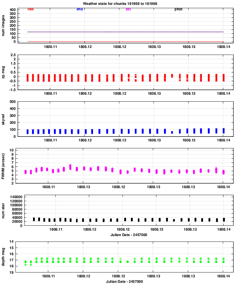
After running the pipeline to reduce the data, clean the images, find and measure stars, calibrate them astrometrically and photometrically, I used a script to look at properties of the data over the course of the night. You can read more about the "weather" in another note.
Below are links to the graphs produced for each of the 4 quadrants.
Quadrant 1:
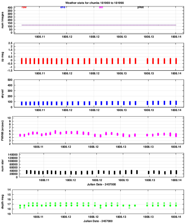
Quadrant 2:
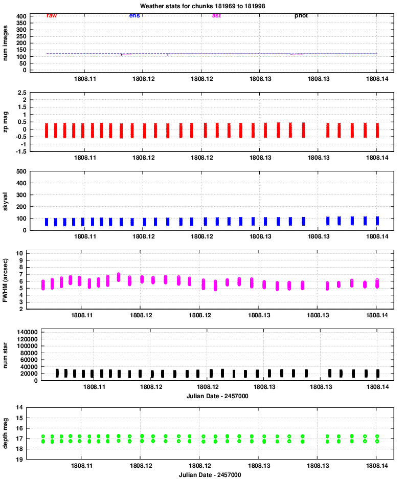
Quadrant 3:
Quadrant 4:
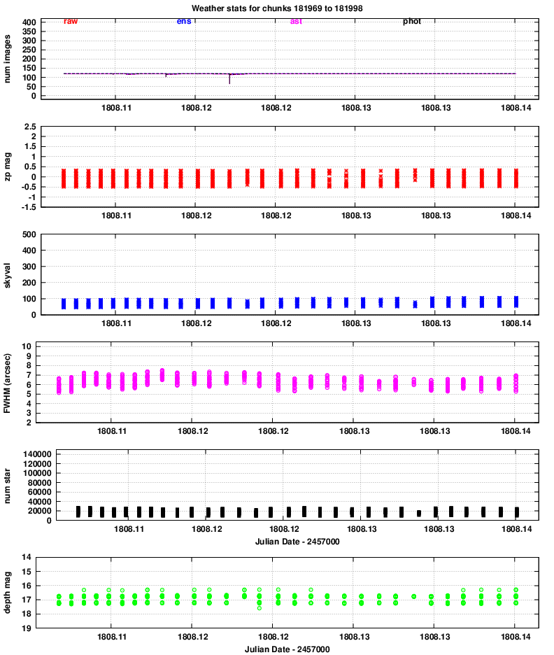
One conclusion is that the properties of images in all 8 chips vary together: when one reports better seeing, they all report better seeing, for example. That confirms that the hardware is working properly.
There are a few chunks missing from the graphs; in each case, there were no chunk datafiles in the original input directory, so my guess is that something happened in the earlier round of processing, before I started examining the data.
Let's go through the panels of these graphs, one by one, and comment on features of interest.
zp = (instrumental_mag) - (calibrated_mag)
Large positive values indicate extinction due to the atmosphere or clouds.
No big changes here.
However, it is clear that the FWHM for quadrants 3 and especially 4 is considerably larger than that of quadrants 1 and 2.
The number is smaller in quadrants 3 and 4, likely due to the larger FWHM and so reduced sensitivity to point sources.
Note that the peak of 40,000 detections per chunk corresponds roughly to (40,000 / 120) = 333 stars in each image. The area of each image is
                2008 x 1128 pixels  =  1701 x 955  arcsec

                                    =  1.63 x 10^6  sq. arcsec

                                    =  451          sq. arcmin

                                    =    0.125      sq. degree
The typical distance between stars is about 70 arcsec, which means that the fields are sparse, not crowded. Aperture photometry should be fine for most stars.
The images typically show stars down to mag V = 17 and a bit fainter. We can see that, again, quadrants 3 and especially 4 have slightly lower quality than quadrants 1 and 2.
After all the data had been calibrated, I ran the "transient_a.pl" script, which applies the rules described in the Tomo-e transient search paper to look for sources with only a brief existence. The code also computes a "control time" for the dataset.
The software found 40, 54, 38, and 27 candidates in quadrants 1, 2, 3, and 4, respectively. I created a web page showing the properties of these candidates in each quadrant:
The entry for each candidate includes some information about the chunk in which it appears, its position in (x,y) pixel coordinates and (RA, Dec) coordinates, and its magnitude. The "variability score" describes the ratio of the standard deviation of its magnitudes away from the mean to the standard deviation from the mean of stars of similar brightness; so, a high score means the object is varying from frame to frame more than most objects of similar brightness.
The entries for quadrants 2, 3, and 4, contain columns listing the magnitudes of any objects at this position (to within 5 arcsec) in the USNO B1.0 (avergage of R-band magnitudes) and in the 2MASS catalog (K-band magnitude). A value of "99.0" indicates that no source appears in the catalog as this position. You can see that the overwhelming majority of candidates do correspond to objects which were detected in one or both of these catalogs -- meaning that they are not true transients.
After these columns of text, the documents contain thumbnails of the images around the candidate. The thumbnails are oriented with North up, East left, and are 110 pixels (= 130 arcsec) on a side.
I found no candidates which looked like real transients in this dataset; feel free to examine them yourself.
The table below shows the control times for each quadrant in this dataset:
quadrant         control time (square degrees * sec)
                   V=13     V=14     V=15     V=16
--------------------------------------------------------
  1                8040     8040     8040     7364
  2                8515     8515     8515     8385
  3                8342     8342     8342     4904
  4                8040     8040     8040     2617

 total            32937    32937    32937    23270
--------------------------------------------------------
The total control time is of order 30,000 square degrees times seconds, down to a limit of V=16 in a 1-second exposure.
These control times are roughly the same size as the control times listed in the transient paper; even though this dataset covers less than an hour (instead of one entire night), it is based on a full set of 84 chips (instead of just 8 chips in the prototype camera).
A single whole night, measured with all 84 chips, should accumulate as much control time as the eight nights analyzed in the transient paper.