I'm an astronomer at the Rochester Institute of Technology, where I teach courses in astronomy and physics, and do some research. My specialty is the analysis of optical images; I've written quite a bit of software for this purpose.
I really enjoy looking for, and studying, celestial objects which CHANGE: stars that move across the sky, or objects that suddenly grow much brighter before fading away. In order to find these interesting sources, and in order to study their evolution, it is necessary to extract quantitative information from digital images.
In this presentation, I'll try to describe a few of the obstacles that we must overcome to do so, and to explain very briefly how to overcome those obstacles. This is not an exhaustive list of the problems that can appear in CCD or CMOS data, and my descriptions will be simplified for reasons of limited time (and, to be honest, probably limited interest in all the gory details).
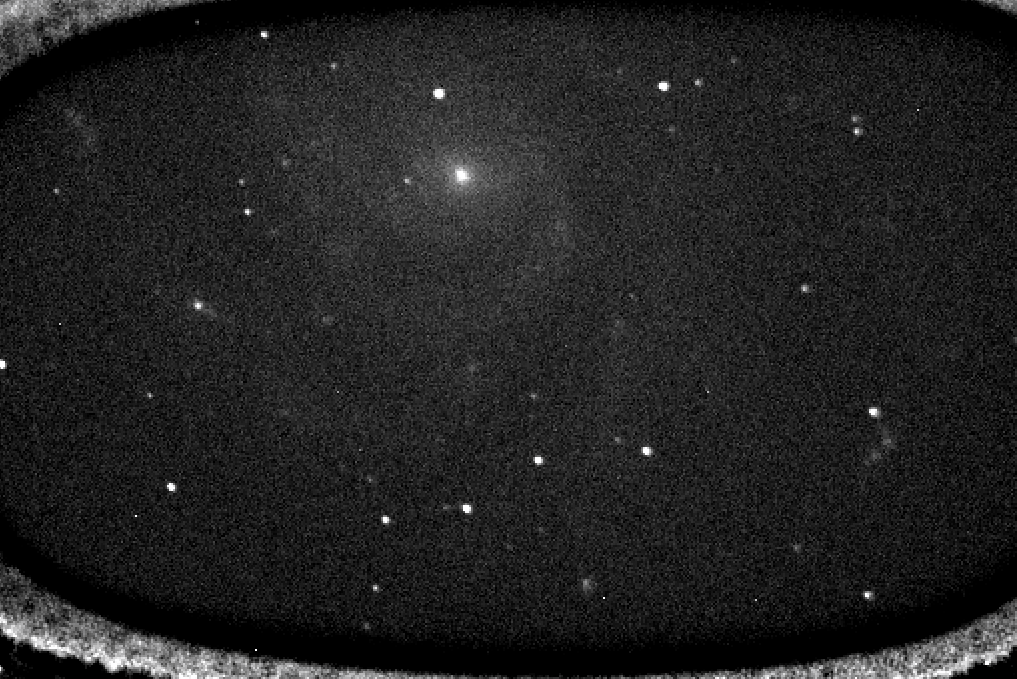
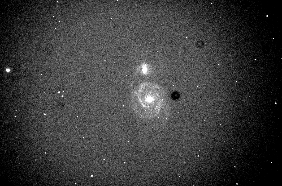
When astronomers take images with their CCD or CMOS cameras, they don't always look very pretty. For example, during a study of an object in the nearby spiral galaxy M101, a typical single image looked like this:
Q: Can you even SEE the galaxy in this picture?
There are at least two obvious types of image defects in that picture:
It's certainly not "pretty", and would never impress anyone who has seen the wonderful pictures from Hubble or JWST -- or those taken by the thousands of skilled amateurs around the world. However, with the proper processing, even a picture as ugly as this can provide solid scientific information. Let me try to give you an idea of the procedures I (and other astronomers) follow in order to spin gold out of this dross.
Solid-state detectors are built around a thin wafer of crystalline silicon, sometimes doped with small amounts of other elements. The basic idea is that when a photon from the sky strikes the silicon, it will knock free one electron from an atom in the crystal; that electron can then be collected with others striking the same pixel, creating a big pool of electrons. By measuring the charge of that pool of electrons, we can determine how many photons struck the pixel.
However, thermal motions of the atoms in the crystal can cause them to bump into each other, which can ALSO eject electrons: this is called dark current, because it produces electrons even when no light from the sky shines on the silicon. Cooling the crystal will reduce these motions, but in some cases, a significant number of thermally-generated electrons will still appear in raw images.
Note that certain pixels are particularly sensitive to these thermal excitations; they may contain small imperfections in the crystalline structure. You can see hundreds of such "hot pixels" in the example above.
Fortunately, the dark current is very consistent: if one takes a series of pictures at the same temperature and exposure time, one will measure nearly identical levels of the dark current. So, to fix the problem,
The result is much cleaner.
After these particular images were cleaned, I was able to use them to measure the distance to Pluto.
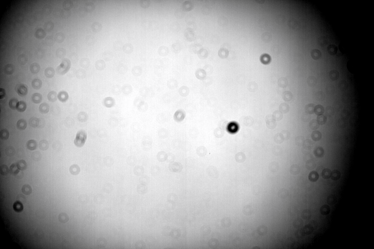
If one takes a picture of a uniformly bright, featureless light source, such as
one ought to see ... a uniformly bright, featureless image. Right?
But in practice, when we take images of such "flat" light sources, we see something different: pictures with gradients from center to edge, as well as dark rings of various sizes.
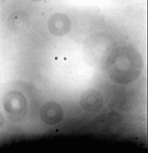
   Q:  What is the cause of those dark rings?  And why are
             some larger than others?
These issues aren't confined to small telescopes; even the cameras at big, professional observatories show these features. The example below comes from the MOSAIC multi-CCD wide-field camera at the Kitt Peak National Observatory. In addition to the grandients and dark rings, one can also see some linear features related to structures of the telescope and the camera.
Image of MOSAIC camera flatfield courtesy of
NOIRLAB
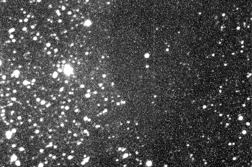
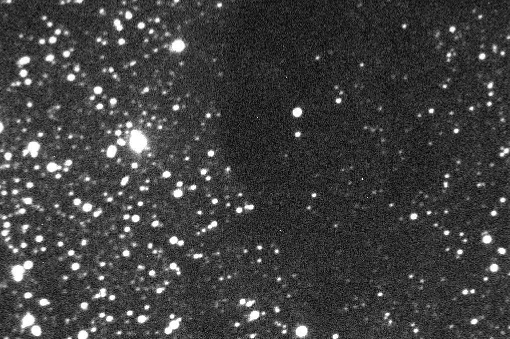
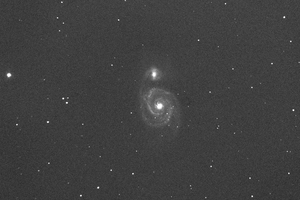
These imperfections show up very clearly when one takes long-exposure images of objects with low surface brightness -- such as galaxies. (Does anyone recognize this galaxy?)
How can we remove these features? It takes just a little extra work. Before (or after) an observing run, we point our telescope at the twilight sky, or an illuminated screen inside the dome, and take a set of pictures: flatfield images. Notice that the locations of the rings in this image match the locations in the target image of the galaxy.
The result will be a picture that not only looks more aesthetically pleasing, but also more faithfully records the relative brightness of objects at different locations in the field.
There are other issues which can appear from time to time in CCD or CMOS images. For example, if one exposures for too long on a very bright target, the pool of electrons in a pixel may grow so large that it starts to overflow and run into neighboring pixels. We call these "bleed trails".
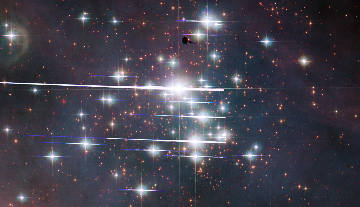
HST image of Trumpler 14 courtesy of
Judy Schmidt
An issue which is most serious for telescopes in space is due to cosmic rays. Photons aren't the only particles which can knock electrons free from their atoms in the silicon crystal: high-energy electrons or protons will do so as well if they happen to smash into the detector. Space is full of these energetic particles, and they show up frequently in images taken by space-based instruments.
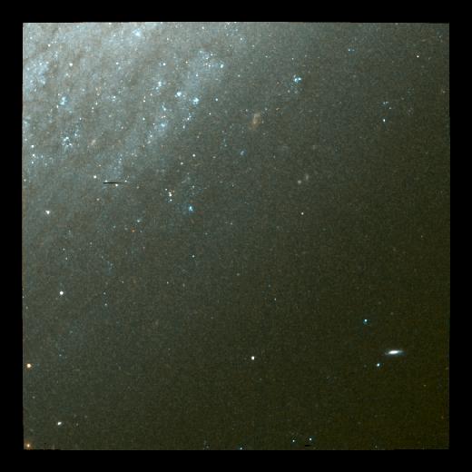
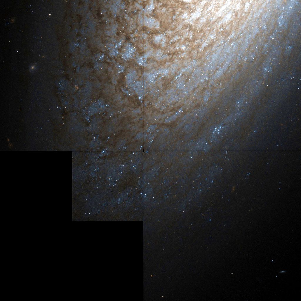
The example below shows an image of a small portion of the galaxy NGC 2841 taken by the Hubble Space Telescope. The big line running nearly vertically through the picture is due to another Earth satellite which just happened to be passing by when the picture was taken -- bad luck. But the many, many smaller streaks and dots are caused by individual electrons and protons running into the Wide-Field Planetary Camera 2 (WFPC2).
Q: How can we remove the streaks caused by cosmic rays?
A good technique is to take multiple images of the target. Each image will include a number of cosmic-ray hits, but the locations of these strikes ought to be completely random. That means that in a set of, say, 5 images, one particular pixel may be contaminated only once. By using a median technique to combine the images, we can discard any individual discrepant pixel values, using only the good pixel values in the output.
For example, I combined just TWO images -- each full of cosmic ray hits -- to produce this much cleaner result.
The larger the number of images used as input, the more pristine the result. I combined 20 images taken through both V-band and I-band filters to create the color composite below.
My example was taken from just one quadrant of the full WFPC2 camera. If one processes all four of them in this way, one can make a very pretty -- and scientifically useful -- mosaic image of the galaxy. These images were part of a project used to determine the distance to NGC 2841 by measuring Cepheid variable stars in its outer regions.
HST image of NGC 2841 courtesy of
WikiSky
Okay, so we have a clean digital image, one in which the intensity of each pixel is proportional to the number of photons which struck it. At this point, we are ready to make quantitative measurements:
Due to our limited time, let's focus on just the first of these questions. To illustrate our point, let's use this image of the spiral galaxy M74. How we can we measure the brightness of the star to its southwest?
![]()
Q: How could we measure the brightness of this star?
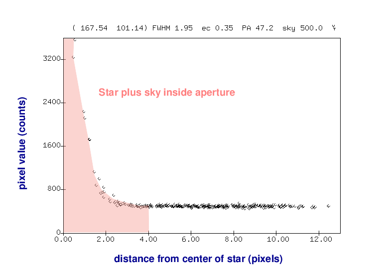
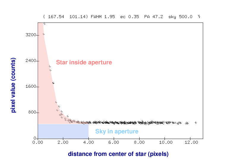
Well, we could define a small circle that is a bit larger than the visible extent of the star, and simply add up all the light inside the circle. Easy-peasy.
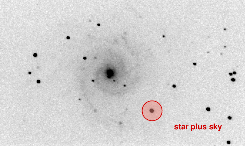
Unfortunately, this will count both the light from the star (which we want) as well as the light from the sky in front of the star (which we don't want).
Therefore, let's make a second measurement: we'll define a region around the star which should include only light from the sky itself.
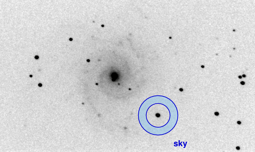
We can use this ring-shaped region to determine the brightness of the sky alone.
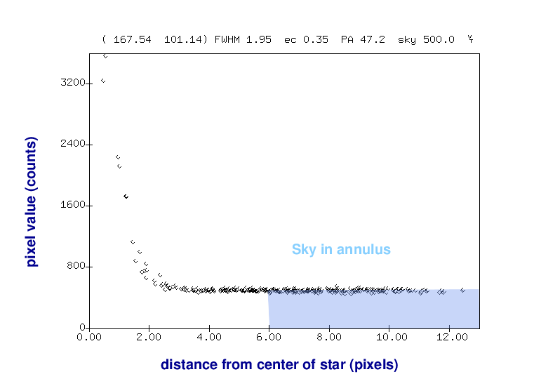
Armed with this information, we can accurately remove the contribution of the sky background from our measurement of the star's brightness.
Most of us aren't lucky enough to take images with a telescope in space, so we have to deal with the complications of ground-based astronomy. One of those involves clouds -- not a big surprise to anyone living in the northeastern US. In order to explain the nature of the problem, and to illustrate the solution, we can use some measurements of this field around the star IY UMa ; it's a cataclysmic variable star which can show strong changes in brightness over periods of just a few hours. The other stars in the field are just ordinary random stars, with no known special properties.
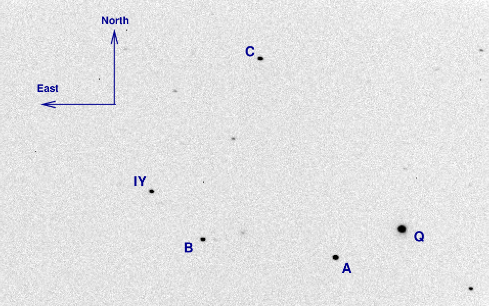
If we use a set of circular apertures and surrounding annuli to measure the brightness of the stars in this area labelled "A", "B" and "IY", we would expect to see ... well, what _would_ we expect to see?
  Q:  What should we see if we plot the brightness of stars A, B
           and IY over the course of several hours?
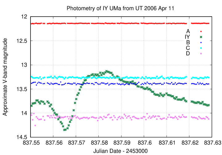
Okay, let's begin. Here are the measurements of the star IY UMa.
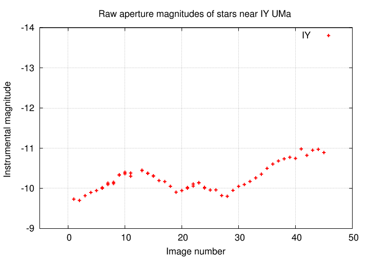
Q: Is the star IY UMa changing in luminosity?
Golly, it surely looks as if the star is growing brighter, then fainter, then brighter, throughout the observing period. Based on this information, we might conclude that IY UMa really does produce a varying amount of power over the course of several hours.
But, just to make sure, let's look at a second object in the same images.
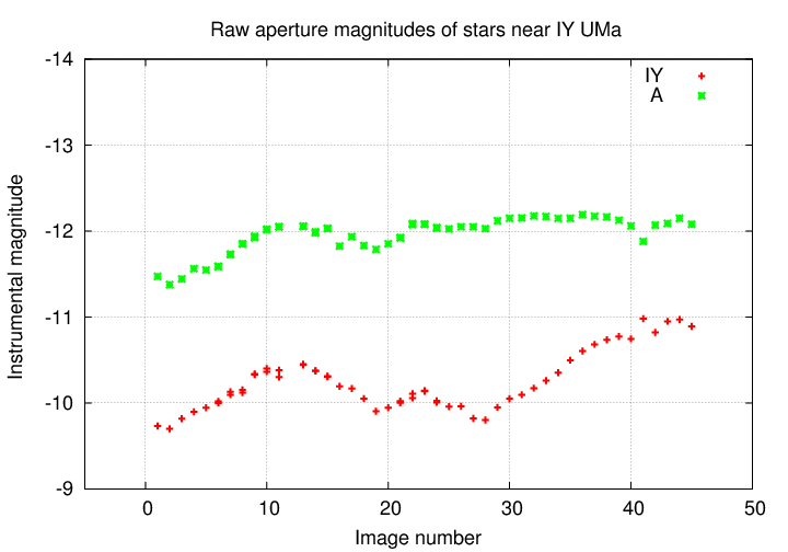
    Q:  Is the star IY UMa changing in luminosity?

    Q:  Is the star A      changing in luminosity?
Hmmmmmmmm. It looks as if both stars are changing in brightness, in almost, but not quite, the same manner. Does that make sense? These two stars aren't really close together in space; why should they be varying in sync?
Well, let's look at the third star we measured, the one called "B".
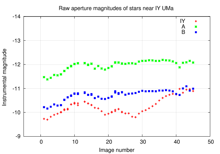
    Q:  Is the star IY UMa changing in luminosity?

    Q:  Is the star A      changing in luminosity?

    Q:  Is the star B      changing in luminosity?
Huh? All three stars just happen to be producing more and then less and then more power, all at the same time? This just doesn't make sense.
Q: What is going on here?
Why should three stars in the same region of the sky all grow brighter and fainter at the same time? While it's possible that they might all have the exact same sort of instability within their atmospheres, affecting them identically, it's much more likely that the culprit is the Earth's atmosphere.
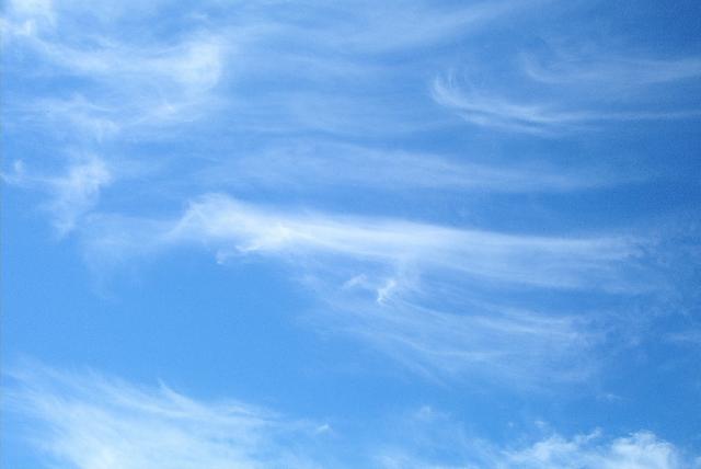
Image courtesy of
Lin Chambers and NASA
If clouds happen to move in front of the tiny patch of sky we are observing, then ALL the stars in that patch will grow dimmer simultaneously; if those clouds then move away, then ALL the stars will grow bright again, simultaneously. To a good approximation, changes in transparency will cause all stars in an image to vary in apparent brightness, in sync with each other.
Well, if we want to measure the REAL variations in one particular star -- variations caused by a real change in the amount of light produced by the star -- those real variations are going to be all mixed up with "fake" variations caused by the atmosphere.
  Q:  Is there any way to isolate the REAL variations
      in one star from these "fake" changes?
Yes! There is a relatively simple procedure which will remove (most of) the changes due to the Earth's atmosphere. All we need to do is to compute the differential magnitudes of stars relative to some reference object. Suppose, for example, that we choose our reference object to be star A. Then we just subtract the instrumental magnitude of star A from the instrumental magnitude of every object:
    diff mag of star A  =  (mag of A)   -  (mag of A)

    diff mag of star B  =  (mag of B)   -  (mag of A)

    diff mag of star IY =  (mag of IY)  -  (mag of A)
Let's look at the results. How much does star A change, relative to star A?
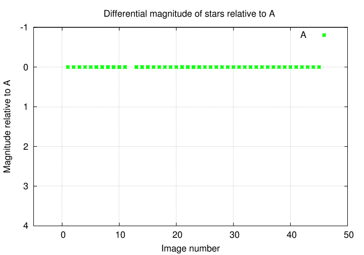
Not at all. Good!
Okay, something more interesting. How about star B, relative to star A?
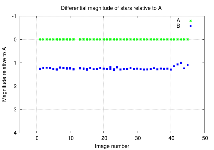
Well, star B seems to be roughly the same brightness relative to star A, with little variations from image to image. There is a bit of a rise near the end, but nothing really convincing.
But if we add IY UMa to the mix ....
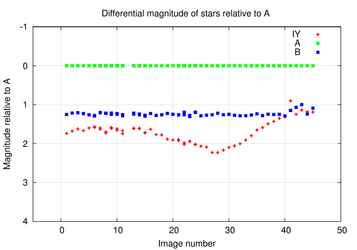
A-HA! Now, this is some strong evidence that the star IY UMa really is producing more light, then less light, then more light again.
Okay, so we now have a set of differential magnitudes for each of our stars.
  Star          differential mag
----------------------------------------
   A               0.00

   B               1.24

   IY              1.90
----------------------------------------
But we'll run into problems if we stop at this point and publish a paper stating that the magnitude of IY UMa in this image is 1.90. We chose to measure our differential magnitudes relative to star A -- but what if we'd chosen star B? In that case, the differential magnitude would be 0.66 -- a very different value.
Differential magnitudes are useful for some purposes, but cause problems for others. In order to make our results as useful as possible to other scientists, we need to put our measurements on some sort of standard system. In other words, we need to calibrate them.
One easy way to calibrate our measurements is to find our reference star in one of the widely used catalogs. For example, the APASS 9 photometric catalog lists magnitudes in the BVg'r'i' passbands for over sixty million stars. The star labelled "A" in our images is entry 5915461 in the APASS 9 catalog:
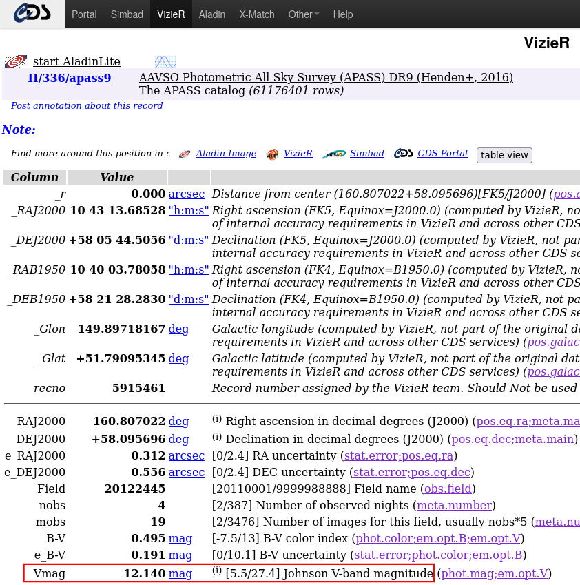
The V-band magnitude of this star is 12.140. To first order (yes, yes, we are simplifying a bit here), we can simply add this catalog value to all of our differential magnitudes to yield the V-band magnitude of each star.
  Star          differential mag      V-band mag
--------------------------------------------------------
   A               0.00                12.14

   B               1.24                13.38

   IY              1.90                14.04
--------------------------------------------------------
And now everyone else will know exactly what we mean when we write that "we measured IY UMa to have a V-band magnitude of 14.04 in this image."
If we apply this method to all of our measurements, in all of the images taken during a night, we can construct a calibrated light curve.
All those steps can take a lot of time and effort; and, for many purposes, they aren't necessary. If you want to create a very nice picture of the Orion Nebula or Jupiter, sure, the first few steps are required, but there's no need to perform all the measurements and calibrations. And that's fine.
But there are cases in which one MUST go through all these reductions (and more, to be honest -- I've simplified a number of them). In particular, if one wishes to share data on a celestial source with other observers, so that the measurements can be combined, careful calibration is absolutely key. Moreover, without calibration, one cannot compare observations to theoretical models properly.
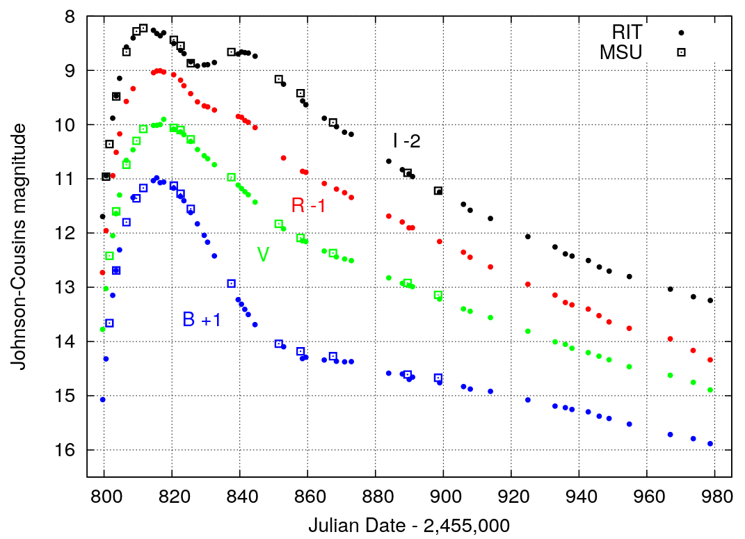
Let me show two examples. The first is a supernova that we saw explode eleven years ago, in 2011. Using our 12-inch telescope at the RIT Observatory, I tried to acquire images every clear night (at least for the first month). The results aren't very pretty
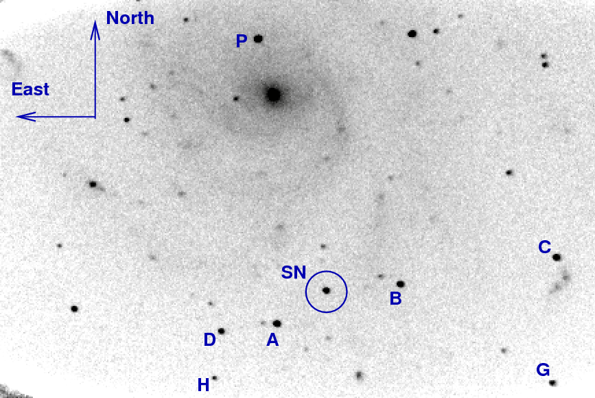
but they did allow me to measure the quick rise and gradual decline of the event at four different wavelengths in the optical.
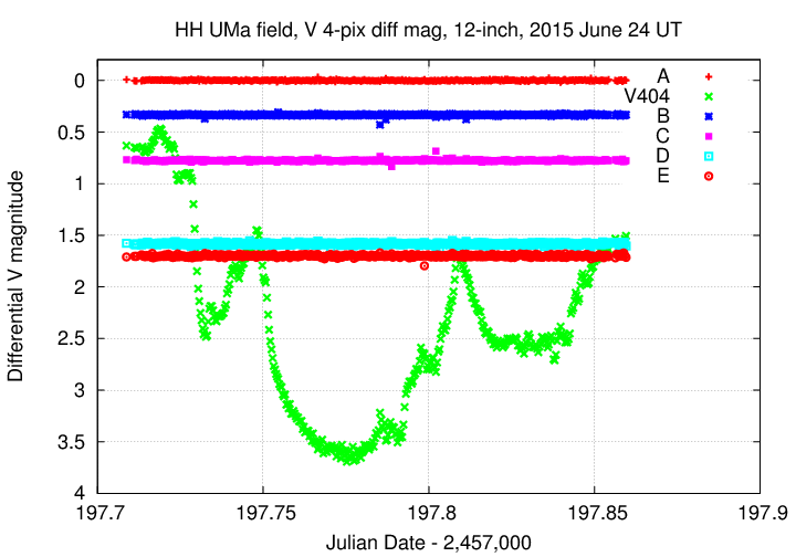
In the summer of 2015, a binary system consisting of a giant star orbiting around a black hole went into outburst: gas in an accretion disk around the black hole suddenly heated up and emitted large amounts of energy across the entire electromagnetic spectrum (X-ray through optical and into the radio) for several weeks.
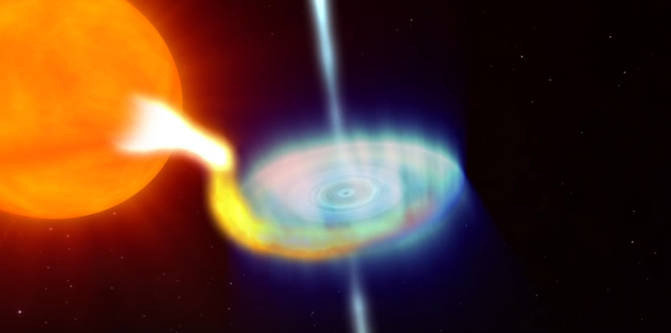
Movie courtesy of
NASA/Goddard Space Flight Center/Conceptual Image Lab
Astronomers around the world -- many of them amateurs with telescopes similar to our 12-inch Meade -- dropped everything else and monitored this system intensely. By combining measurements taken at different locations on Earth, we were able to produce a nearly continuous record of the system's evolution in luminosity over the outburst.
I was watching on the night of June 23/24, 2015, when the variation went crazy.
During a span of just three-and-a-half hours, the system's optical luminosity dropped by 3.5 magnitudes (down to just 4 percent of its starting value), then recovered and rose back up to just 1 magnitude (40 percent) of its original value.