 Copyright © Michael Richmond.
This work is licensed under a Creative Commons License.
Copyright © Michael Richmond.
This work is licensed under a Creative Commons License.
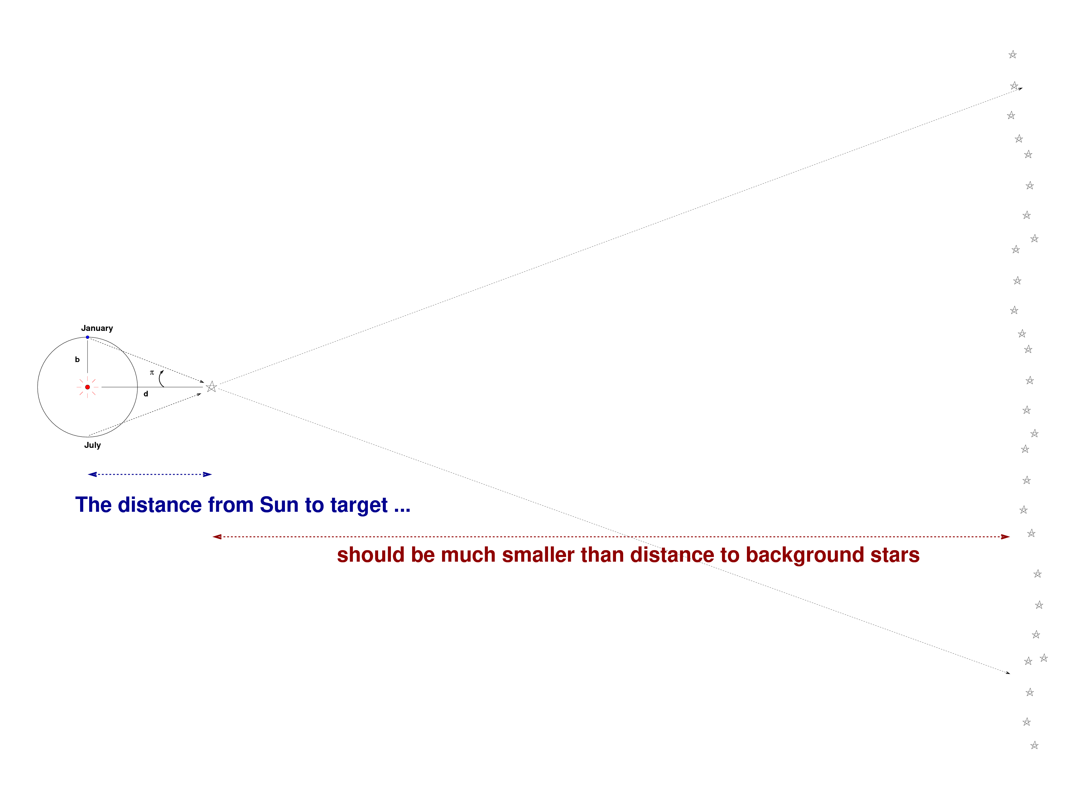
Parallax is the apparent shift in position of a nearby object when it is viewed from different locations. Those might be two different observatories on the Earth's surface (as was the case in the famous transits of Venus in the eighteenth and nineteenth centuries), but, in most astronomical applications, are two spots in Earth's orbit around the Sun:
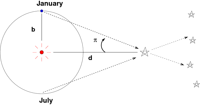
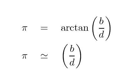
If one knows the value of the baseline distance b, and can measure the parallax angle π
Yes, I know this is confusing. Yes, astronomers back in the old days should have picked a better letter. Sometimes you see the "curly pi" used to denote this angle, but few font families include it
then one can use simple geometry to compute the distance to the target object d.
Q: Write a simple formula for d.
Of course, that simple formula ignores many complications. For example,
But one can work around these issues, or at least place constraints on their consequences.
The importance of parallax lies in its fundamental simplicity: we humans understand geometry, and trust it. As long as we can make measurements of the angular displacements over time, we can use the resulting distances with confidence.
There may be minor issues involving corrections for the small shifts of the background reference stars themselves; but if we choose to use galaxies or quasars as the reference sources, we can avoid those completely.
Most important of all, parallax is a direct method of measuring distances. It relies on a single assumed quantity: the astronomical unit (AU) = the distance from Earth to Sun. Back in the 1800s and early 1900s, this was indeed a major issue, and astronomers great efforts to pin down the value of the AU. But these days, thanks to radar and spacecraft flying through the solar system, we do have a very, very good idea for the size of the AU. For example, the JPL Horizons system uses a value taken from the Planetary and Lunar Ephemerides DE430 and DE431, which list
1 AU = 149597870.700 km
That's ... quite a few signficant figures.
And that's it. Heliocentric parallax does NOT require any assumptions about stellar luminosity or evolution, or the distribution of sizes and colors of stars, or the spectral energy distribution of glowing hydrogen gas.
So, if astronomers can measure a distance via parallax, they will rely on it much more than distances determined by other methods.
So, parallax is a good method. But how far out into space can it reach?
Back in the old days, when parallax was performed by optical telescopes from the surface of the Earth, it was very difficult to achieve precisions of better than about 0.01 arcsec. Let's use milliarcseconds (mas) from this point forward, as it will be more convenient. So, good ground-based measurements had precisions of perhaps 10 mas.
The very best, made with specially-built instruments such as the Multichannel Astrometric Photometer at Allegheny Observatory , could achieve precision of 1 mas for a few stars, after many observations.
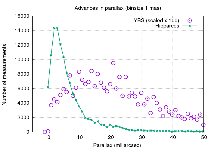
However, no such devices could make all-sky surveys. As a result, catalogs of stellar distances were incomplete, as well as being rather low in precision. For example, the Bright Star Catalog , compiled over the period of 1964 to 1991, listed parallax values for about 2700 stars.
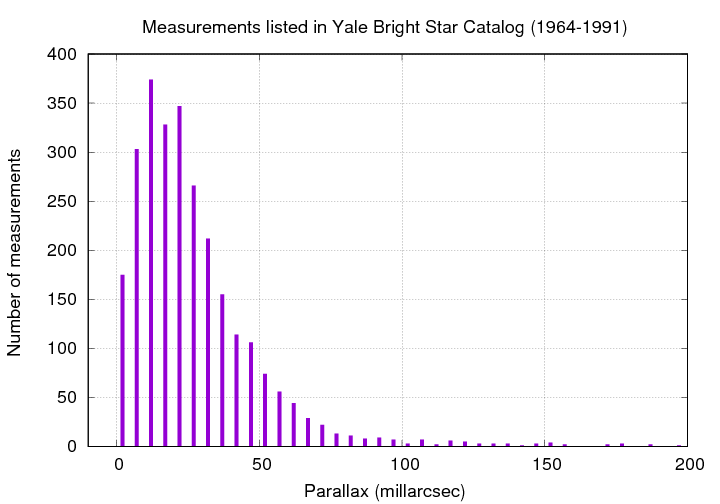
  Q:  What is the most common value for parallax (mas)?


  Q:  If we could measure stars perfectly, what should
            the most common value be?
The fact that this histogram turns over below 15 mas is a sign that the precision of the typical measurement is ... about 15 mas.
  Q:  If the uncertainty of a typical measurement is
            15 mas, how far away can a star be
            and still have a "good" distance?
It turns out that the nature of parallax measurements means that the connection between the error in the measurement and the error in the distance is not simple. There are a number of tricky aspects which can make the analysis of, say, the possible bias in some catalog, a complicated matter.
The first big problem is that the quantity of interest, the distance to a star d, is INVERSELY related to the measured angle π.
This means that an error of (for example) 20 percent in the measurement does NOT mean that there will be an error of 20 percent in the computed distance.
Why not? Well, let's do an example to find out. Suppose that we measure the parallax to a star to be

If the uncertainty is the usual "1-sigma" variety, then this measurement means that the true value of the parallax angle has a 66% chance of lying in the range 80 to 120 mas.
        angle < 80 mas                 16% probability

        80 mas < angle < 120 mas       66% probability

        120 mas < angle                16% probability
Fine so far. But what does that mean for distance we derive from this angle? We need to calculate the distance corresponding to the angle (100 - 20) and the angle (100 + 20). I'll let you fill in the table below.
                  distance <  ___ pc       16% probability

        ___ pc  < distance <  ___ pc       66% probability

        ___ pc  < distance                 16% probability
The fundamental issue here is that a realistic, symmetric error in the measured angle leads to an ASYMMETRIC error in the derived distance. The larger the fractional error in parallax angle becomes, the more asymmetric this error in the derived distance. For example, if we measure
then the range of distances consistent with the measurement at 1-sigma looks like this:
We can sum up this first problem: symmetric errors in a measured parallax angle lead to asymmetric errors in the derived distance ... with a larger range of possible true distances on the "farther away" side.
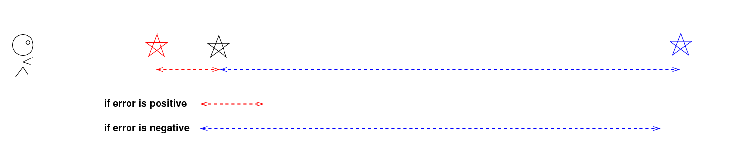
The really nasty bit of the errors-in-parallax discussion is a consequence of the first conclusion: symmetric errors in angle lead to asymmetric errors in distance. Let's go back to this example again:
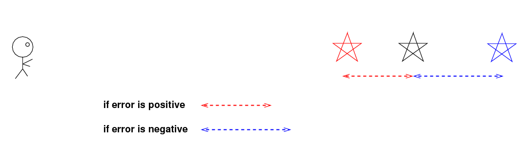
Based on the parallax angle π = 10 mas, we derive a distance of d = 100 pc --- but due to the uncertainty in the angle, the true location of the star has a 66% chance of lying anywhere within the range of 59 - 333 pc.
What that means is that the TRUE location of the star could be here ...
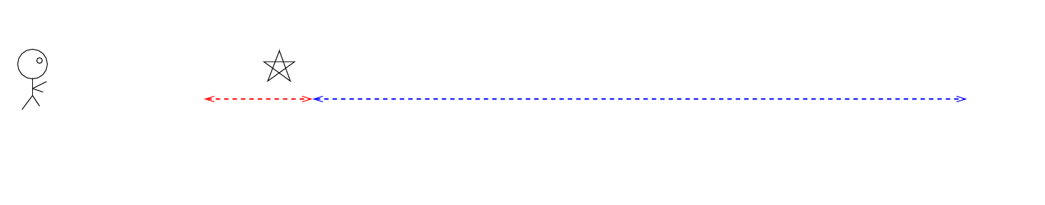
or here
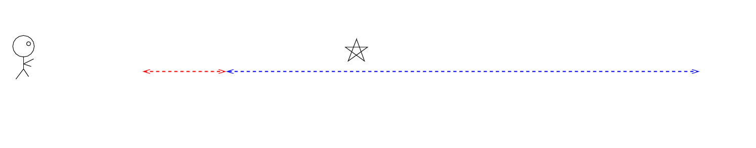
or here

In fact, the star could lie anywhere along a line in this direction, with equal probability, based on that one measurement. In a one-dimensional universe, the probability that the TRUE location of the star is farther than 100 pc is larger than the probability that the star is closer than 100 pc, simply by the ratio of the lengths of the possible locations:
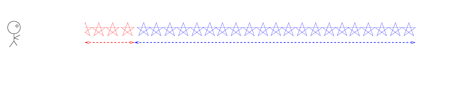
    true location is closer      length  100 -  59  =   41 pc

    true location is farther     length  333 - 100 =   233 pc


    probability that star is farther than 100 pc      333 - 100
   ---------------------------------------------  =   ---------  ~  5.7
    probability that star is closer  than 100 pc      100 -  59
In a TWO-DIMENSIONAL universe, the probabilities would change because the region in which a "farther-than-100-pc" star could exist becomes much larger than that of a "closer-than-100-pc" star.
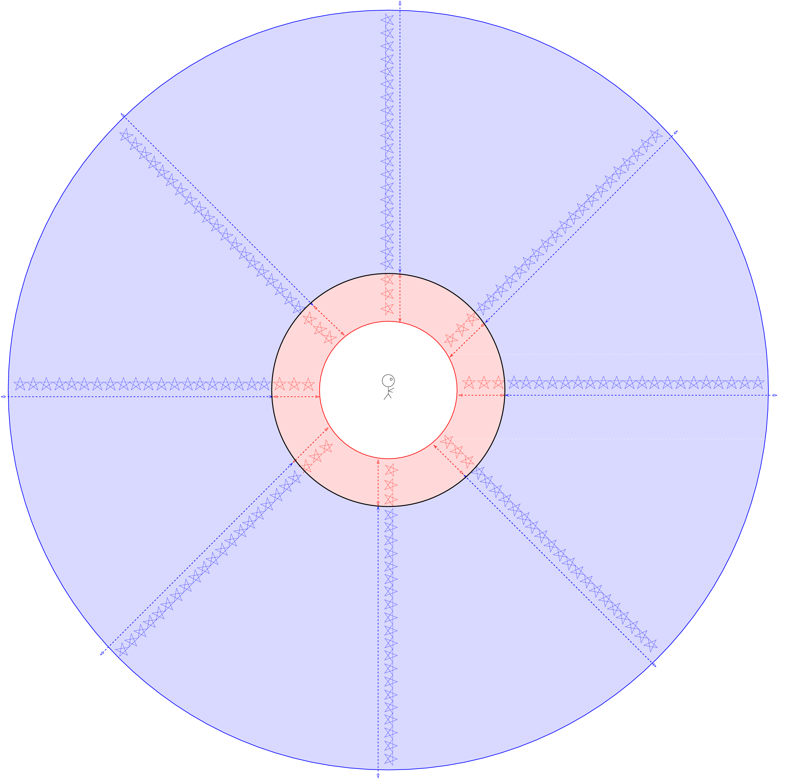
  Q:  What is the ratio of probabilities now?


    probability that star is farther than 100 pc
   ---------------------------------------------  =
    probability that star is closer  than 100 pc
Our course, our real universe is THREE-DIMENSIONAL. Sorry, I can't draw a good 3-D figure showing the two regions, but I hope you can extrapolate from the two-dimensional case to the three-dimensional one.
  Q:  What is the ratio of probabilities now, in 3-D?


    probability that star is farther than 100 pc
   ---------------------------------------------  =
    probability that star is closer  than 100 pc
Now, what's the big deal about all of this? The big deal is that we live in a region of relatively uniform stellar density. In our neighborhood of the Milky Way, there are roughly equal numbers of stars in all directions: left, right, up, down, forward, back. Yes, there tend to be more stars in the plane of the Milky Way, but the thickness of the disk is (until Gaia) larger than typical distance we could measure via parallax, that doesn't really matter.
And so, suppose that we measure the parallax to a star to have the value 10 +/- 1 mas, corresponding to a measured distance of 100 pc. But there are three possibilities for the TRUE distance to this star:
Which of these is most likely? The answer is "C". Because there are more stars in the "more distant" volume, it is more likely that a distant star has been improperly measured than a nearby star. The result is that our measurements of parallax lead to a systematic bias: stars appear closer than they really are (sort of like dinosaurs.)
This effect was noted long ago, by Trumpler and Weaver (1953), among others, but Lutz and Kelker first analyzed it detail in 1973. Astronomers sometimes refer to this bias, or the corrections needed to account for it, as the "Lutz-Kelker effect."
The size of this bias depends (mostly) on the ratio of the uncertainty in parallax to the value of parallax:
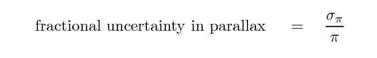
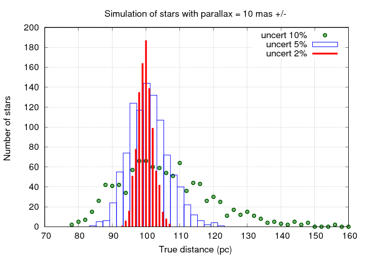
Let's look at some examples. We will observe a set of stars with measured parallax angles of exactly 10.0 mas, which means measured distances of exactly 100 pc.
When the fractional error is very small -- just a few percent -- then the errors in the derived distances, and the overall bias, are pretty small.
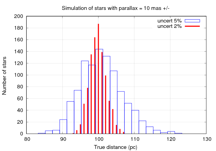
But as the fractional uncertainty grows, the errors and bias increase. Even uncertainties of just 10% can cause big mistakes in the measured parallax. Notice the long tail of true distances out to 140 pc and beyond; the errors in those derived distances are 40 percent or more, far larger than the 10% uncertainty in the parallax angle itself.
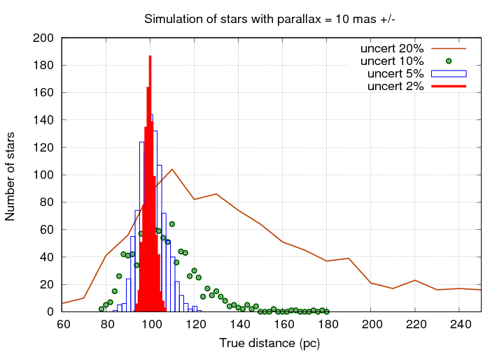
If the uncertainty becomes 20% or larger, the results involve errors which are frequently a factor of 2 or more. No one should try to use such measurements for any careful calculations.
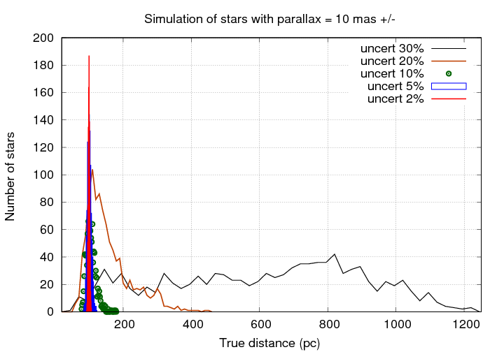
Things are just silly when the uncertaity is 30%!
This table summarizes the results of a simulation in which I created a region of space with uniform stellar density, "measured" enough stars to find 1000 falling within a particular range of parallax values around 10 mas, and then compared those "measured" distances to the actual distances.
       Results of simulations with unform stellar density
           Stars with a measured parallax π = 10 mas
             and a measured distance of 100 pc

  uncertainty            actual distances (pc)
    σπ                mean       median      IQM        IQ range
   ------------------------------------------------------------------
   0.1  =  1%        100.04      100.09     100.06      0.78
   0.2     2%        100.33      100.30     100.27      1.55

   0.5     5%        101.60      101.27     101.29      3.87
   1.0    10%        106.95      105.26     105.57      8.95

   2.0    20%        162.8       143.3      146.9      39
   3.0    30%        626         662        645       221
   ------------------------------------------------------------------
The moral of this story is -- don't trust distances based on parallax unless the uncertainty in the measurement is much smaller than the measurement itself. I would prefer not to rely on any measurements in which the fractional uncertainty is larger than 10 percent.
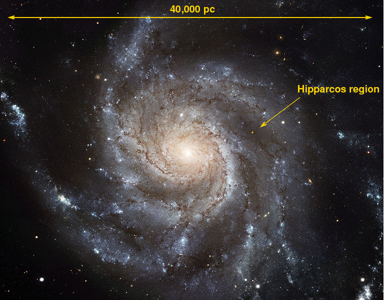
Phew. Now that we understand the weaknesses of the parallax method, we can try to answer this question. If we adopt as a general rule that most ground-based measurements of parallax had uncertainties of about σπ = 10 mas, then we can place a very rough limit on the distances of stars derived from such measurements:
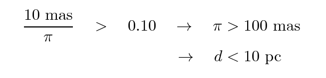
Gosh, that's not very far.
Of course, astronomers DID use parallax measurements which were considerably smaller than 100 mas; scientists are always interested in pushing the limits of their data. But this is a warning that any statistical inferences based on ground-based measurements of stars at greater distances must be very carefully considered, and corrections must be made for the Lutz-Kelker effect.
The Hipparcos satellite was launched in 1989 and its first catalog was released in 1997. This project immediately improved our knowledge of stellar distances (and motions, and luminosities) by a large amount. Not only did it cover the entire sky, and measure stars fainter than those typically found in parallax catalogs (down to about mag 10), it also had a typical precision of about 2 mas. In other words, its typical measurement was about as good as the very best ground-based measurements.
  Q:  If the uncertainty of a typical measurement is
            2 mas, how far away can a star be
            and still have a "good" distance?
One of the wonderful results of Hippacos' measurements were the very accurate HR diagrams which could finally be made, since we now had LOTS of distance measurements to stars of all types. Below is one made using Hipparcos stars with uncertainties of ≤ 10% in their parallax angles.
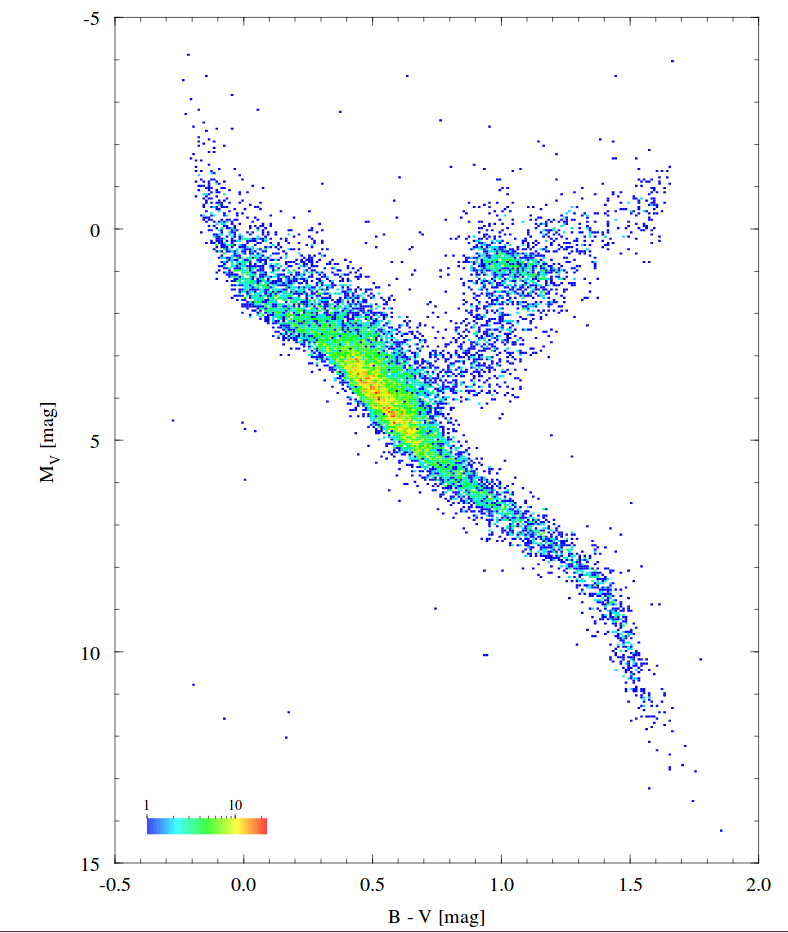
Image courtesy of
ESA's page with HR diagrams based on Hipparcos data.
  Q:  How many different features can you identify
         on this HR diagram?
Gaia is a rather unusual "telescope," since it has been specially designed for astrometric observations. It resembles the Hipparcos satellite in many ways. The basic structure is built around two triple-mirror telescopes which point at regions in the sky separated by an angle of about 106.5 degrees.
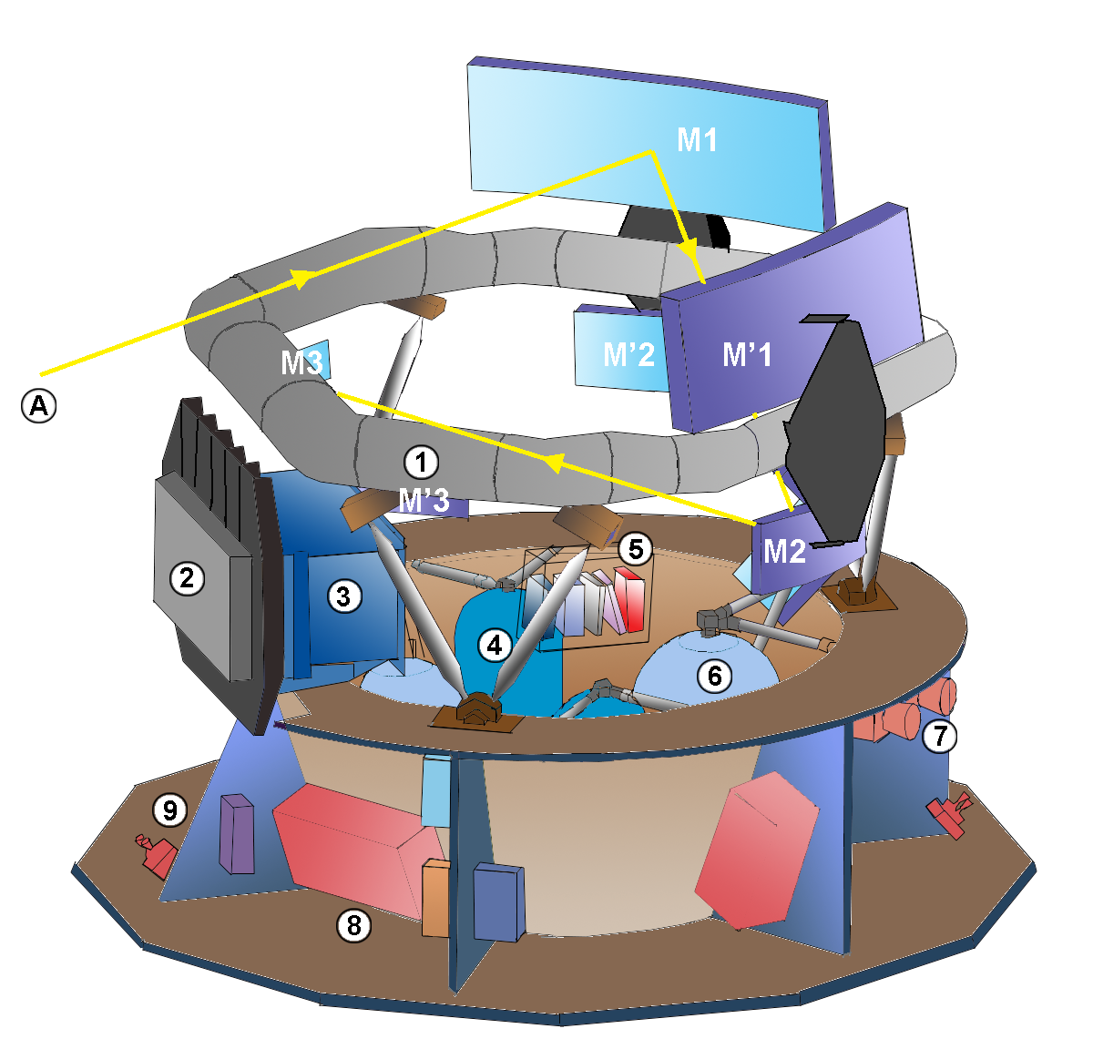
Image courtesy of
Wikipedia
Light from the two telescopes is combined so that it falls upon the focal plane simultaneously. The telescope rotates with a period of six hours, causing stars to sweep across this focal plane in about 60 seconds. Objects in both directions are detected and measured together.
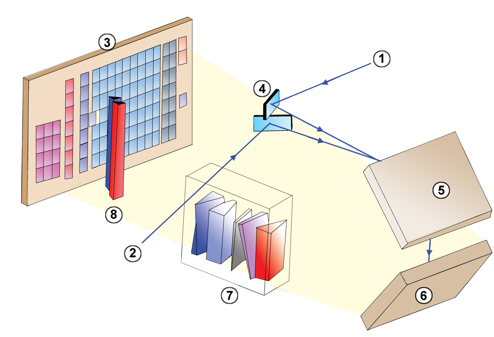
Image courtesy of
Wikipedia

Figure 1 from
Lindegren et al. 2016. Note that this figure
is rotated by 180 degrees relative to previous schematic.
The original caption follows.
Layout of the CCDs in Gaia's focal plane. Star images move from left to right in the diagram. As the images enter the field of view, they are detected by the sky mapper (SM) CCDs and astrometrically observed by the 62 CCDs in the astrometric field (AF). Basic-angle variations are interferometrically measured using the basic angle monitor (BAM) CCD in row 1 (bottom row in figure). The BAM CCD in row 2 is available for redundancy. Other CCDs are used for the red and blue photometers (BP, RP), radial velocity spectrometer (RVS), and wave- front sensors (WFS). The orientation of the field angles η (along-scan, AL) and ζ (across-scan, AC) is shown at bottom right. The actual origin (η, ζ) = (0, 0) is indicated by the numbered yellow circles 1 (for the preceding field of view) and 2 (for the following field of view).
The telescope slowly precesses, so that its spin sweeps out new areas in the sky over time. A typical star will be measured about 70 times over the course of the primary mission (2014 - 2019); that's about 14 measurements per year, though not all equally spaced.
Image courtesy of
Space Flight 101
As the spacecraft precesses, the "partners" of each star will gradually change. Eventually, the spacecraft will have many millions (billions?) of measurements of the relative positions of millions of stars. Scientists can then use a honking-big linear algebra procedure to solve simultaneously for the positions and motions of each star.
How precise are the measurements made by Gaia? As described in Lindegren et al. 2016, the Gaia Data Release 1 consists of a limited set of measured properties for a very limited set of bright stars. Later releases will contain (much) better data for (many) more stars.
   Q:  What is the CURRENT standard uncertainty in the
           parallax for a bright star in DR1?
           Look in Table 1 or Figure 7 of  Lindegren et al. 2016

   Q:  Using that uncertainty, how far out into space
           will Gaia make good distance measurements?
Gaia provides astronomers with many, many more stars than Hipparcos did, so it is possible to create much more detailed HR diagrams:
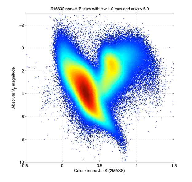
Image courtesy
ESA/Gaia/DPAC/IDT/FL/DPCE/AGIS
As time passes, and Gaia continues to scan the skies, it will build up larger and larger sets of measurements of each star, allowing it to create a better solution for the position, parallax, and proper motion of each object. A recent paper by de Bruijne, Rygl and Antoja provides some predictions for the FINAL Gaia precisions.
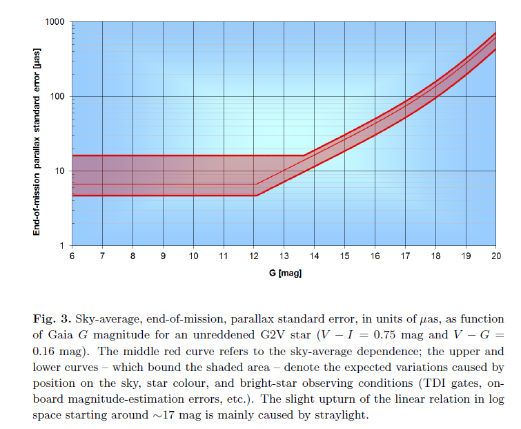
Fig 3 taken from
de Bruijne, Rygl and Antoja (2015)
   Q:  What is the prediction for the FINAL standard uncertainty
           in the parallax of a bright star, when Gaia
           finishes its survey?
           (Look in the figure above)

   Q:  Using that uncertainty, how far out into space
           will Gaia make good distance meausurements?
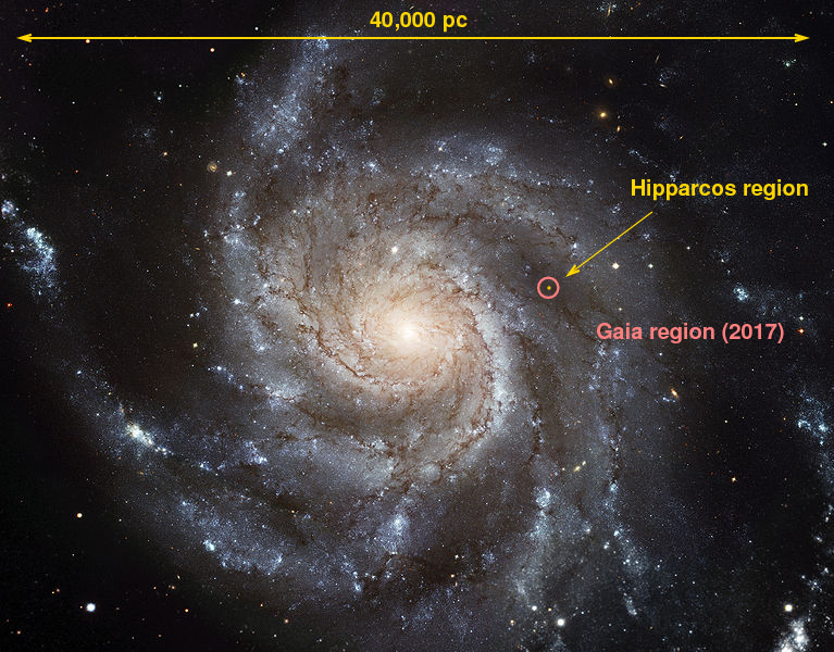
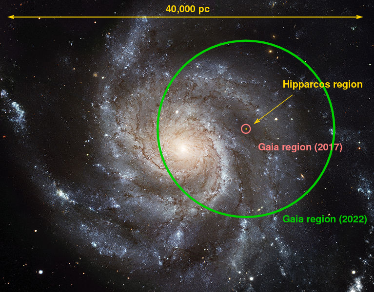
In any case, Gaia will greatly increase our knowledge of the stellar neighborhood. It will produce a catalog of roughly 100 million stars with distances good to about 10 percent. The Hipparcos catalog contains only 0.12 million entries, of which only about 0.04 million satisfy the Lutz-Kelker criterion.
Let's look at the timeline for Gaia operations and data releases.
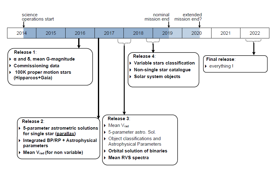
Figure 8 taken from
Eyer et al., 2015
As we will see in a future lecture, the star RR Lyrae is a very important one. It is one of the nearest and brightest of a class of pulsating stars which can help us to measure distances not only within the Milky Way, but to other galaxies.
Clearly, if we wish to use the class of RR Lyr stars as distance indicators, we need to know very precisely how luminous they are ... and, so, how far away they are. Let's consider the star RR Lyr itself.
This is, of course, just one star. But if our estimates of the distances to other stars, and other galaxies, depend upon RR Lyr stars in particular, and if the new Gaia data suggests that our old value might be incorrect by such an amount ... well, that should make you start to worry about the upper rungs on the Cosmological Disetance Ladder!
Based on the earlier discussion of errors in parallax , we might expect that the Hipparcos measurements, with their larger uncertainties, would show a systematic bias relative to the more precise Gaia values. Let's put that to the test.
I went to the Gaia DR1 archive site and chose the "ADQL Search Form", which allows the user to enter SQL-like queries to a number of catalogs.

Into the query box, I entered
  select g.hip, g.ra, g.dec, g.parallax, g.parallax_error, g.phot_g_mean_mag,
            h.hip, h.hpmag, h.plx, h.e_plx
  from gaiadr1.tgas_source as g
            join public.hipparcos as h on g.hip = h.hip
  where g.ra > 0 and g.ra < 359 and g.dec > -90 and g.dec < 90
The result was a set of about 93,000 stars measured by both Hipparcos and Gaia. I then compared the parallax values on a star-by-star basis. As the graph below shows, Gaia and Hipparcos do agree very well, on average: the red dots are individual stars, and the blue symbols are medians within bins of width 1 milliarcsec.
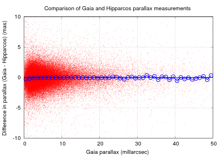
If we zoom in, however, we can see some asymmetry: the Gaia parallax angles tend to be SMALLER than the Hipparcos angles, and the difference grows as the angles decrease in size.
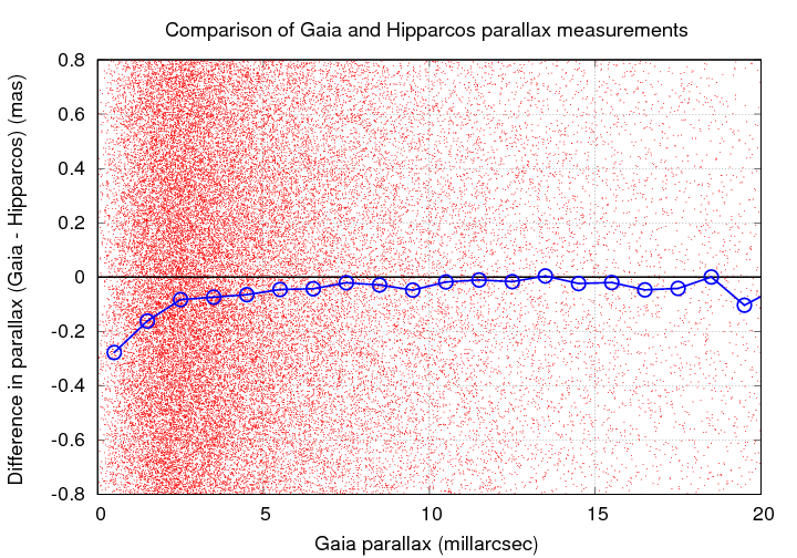
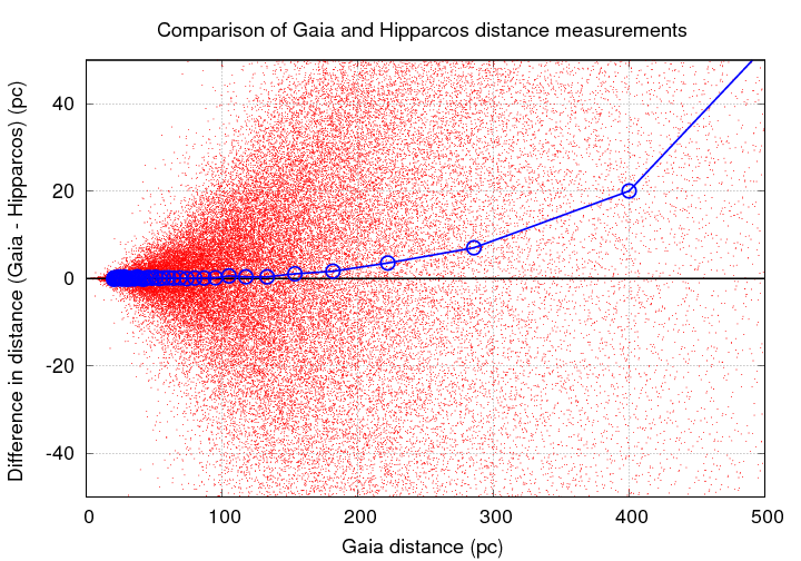
In other words, since the Hipparcos angles are slight OVER-estimates (due to the Lutz-Kelker bias), the Hipparcos distance values tend to be UNDER-estimated as on approaches the limit of its measurements.
We can see that clearly if we plot DISTANCES on our graph instead of angles.
Of course, optical telescopes are not the only ones which can make parallax measurements. Any telescope on (or around) the Earth will share the annual journal, and so have a chance to measure the parallactic shifts of celestial sources.
Stars emit most of their energy in the optical region of the spectrum, and very little in the radio; it isn't possible to detect most stars with radio telescopes. Clouds of gas and dust do emit plenty of radio waves, but they are for the most part large, extended sources, not the compact objects one requires for parallax measurements.
However, there are some circumstances which do allow radio astronomers to apply the power of interferometry to make very precise measurements of the positions of compact radio sources, and therefore to determine the distances to those sources via parallax. The key element is the maser emission from small clumps of gas within some star-forming regions. Astronomical masers arise within compact volumes, thus appearing as point sources to our radio telescopes, and produce radiation of very pure frequency. The combination allows astronomers to determine their positions with very small uncertainties.
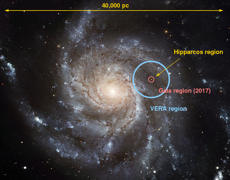
One example of parallax measurements in the radio regime is provided by the Japanese VERA project. VERA is a array of four radio dishes stretched out across the Japanese archipelago.
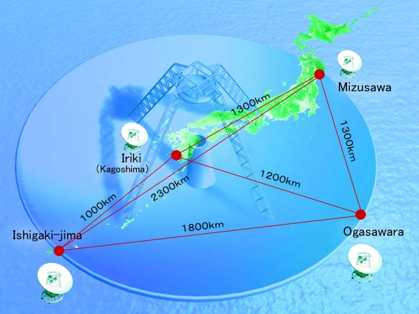
Image courtesy of
The VERA group and the National Astronomical Observatory of Japan
If one looks at star-forming regions, such as S269, with an optical telescope, one sees clumps of stars immersed in gas and dust. If one looks with a radio interferometer, one can see much finer details. Compare the scales on the IR picture at left with the VERA map at lower right.

Image taken from
a presentation by Mareki Honma, NAOJ
If one measures the position of one of these masers over a period of several years, one will see an intriguing pattern. Shown below are VERA measurements of a maser in the Orion-KL region; the figure shows the Right Ascension component of the position as a function of time.
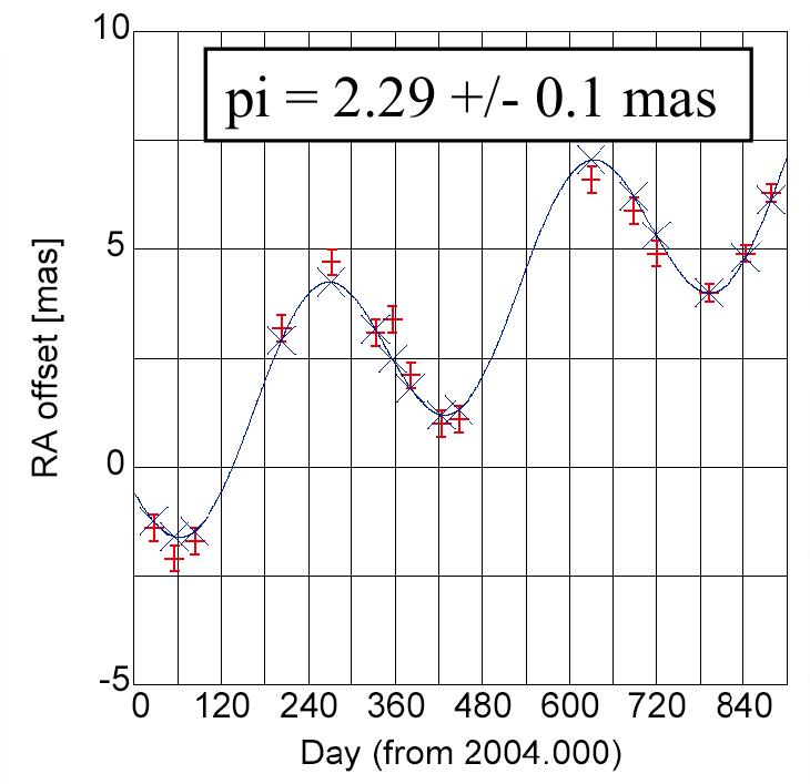
Figure taken from
a presentation by Mareki Honma, NAOJ ;
I've erased the parallax result so that my students can't
peek at it in class.
  Q:  What is the parallax to Orion KL
      based on the measurements above?


  Q:  What is the distance to Orion KL?
A slightly more recent measurement by VERA yields the even more precise parallax to Orion-KL of
Now, if VERA can measure parallax with a precision of 0.03 mas, then it can reach far out into the Milky Way, too. In fact, at the moment, VERA is one of our best tools for measuring distances in the Milky Way, beating Gaia quite handily.
Copyright © Michael Richmond.
This work is licensed under a Creative Commons License.