This little presentation discusses recent measurements of the Milky Way's rotation curve, concentrating on efforts by two groups using very different methods.
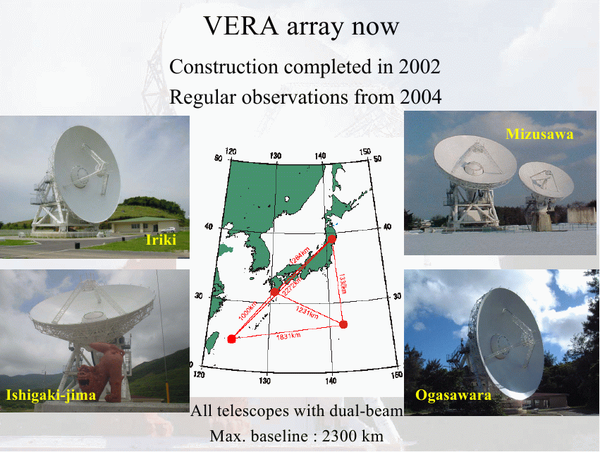
The VERA (VLBI Exploration of Radio Astrometry) team observes microwave emission from celestial masers. There are four antenna scatted across Japan.

One of their targets are masers in the star-forming region S269:
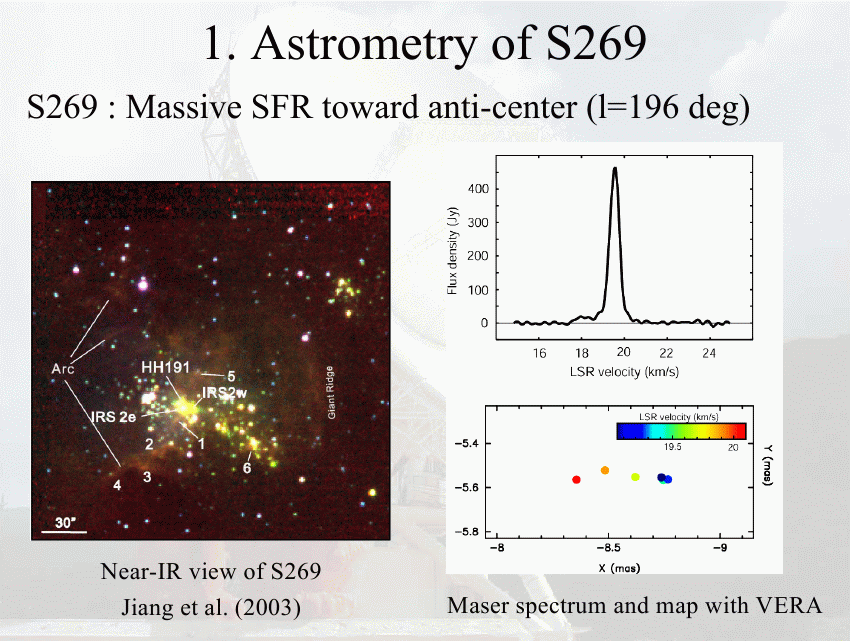
Measurements over a period of slightly more than one year reveal the parallax motion of several of the brightest spots.
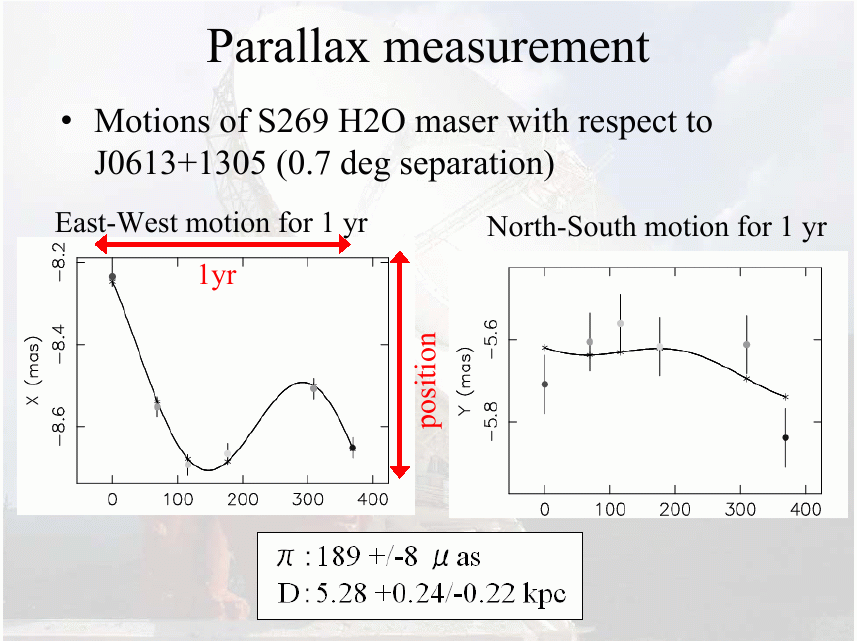

With the distance to the maser source, and the radial velocity of the maser source, and the proper motion of the maser source, we can figure out the source's space velocity and position within the Galaxy.
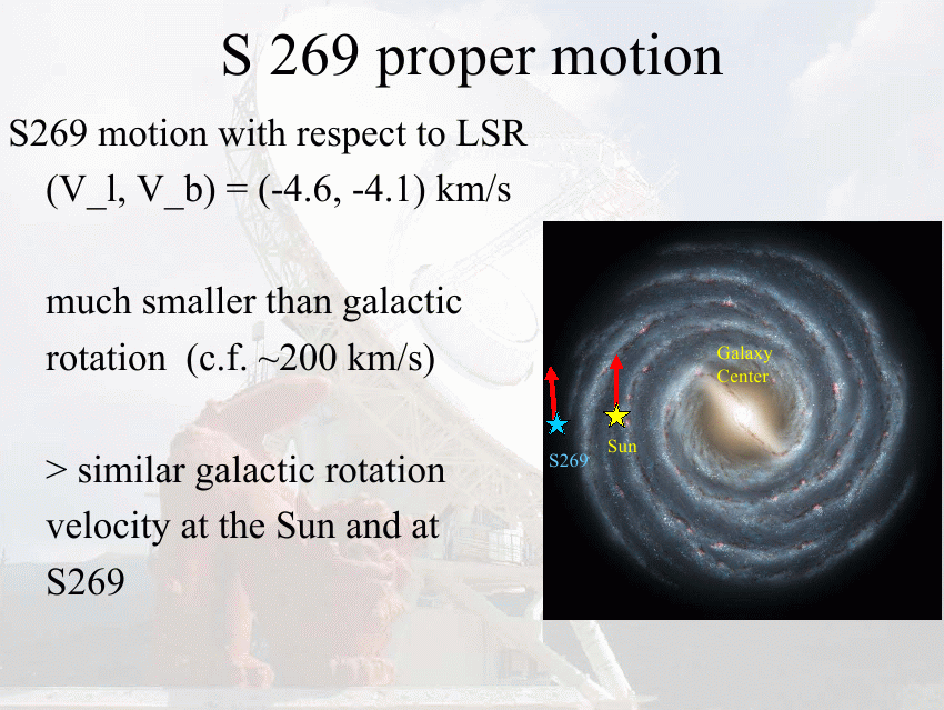 It yields one very precise point on the galaxy's rotation curve:
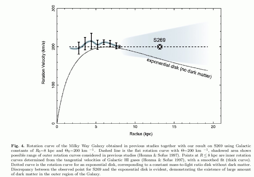
Note that this is only the first such measurement by VERA, but others will come in time:
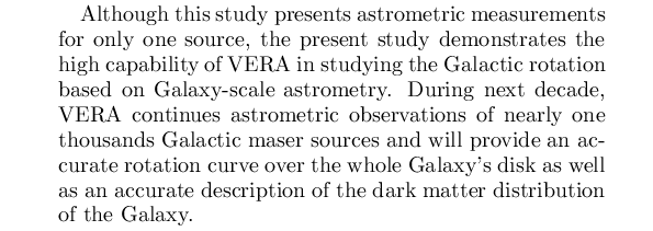
For example, the VERA team is already measuring other star-forming regions:
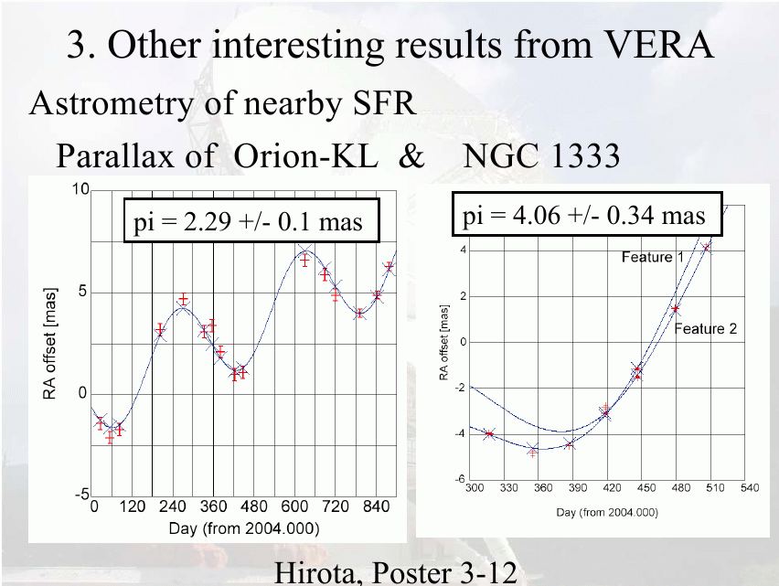
A very different approach is taken by a large team of astronomers sifting through some results from the Sloan Digital Sky Survey (SDSS). They choose Blue Horizontal Branch stars (BHB) as tracers of the galactic potential. Why?
They use color-color plots as the FIRST step in choosing targets ...
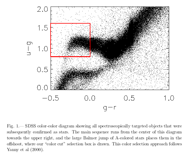
... and spectra for a SECOND step in removing contaminating stars from their BHB sample:
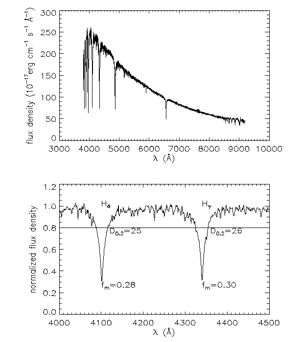
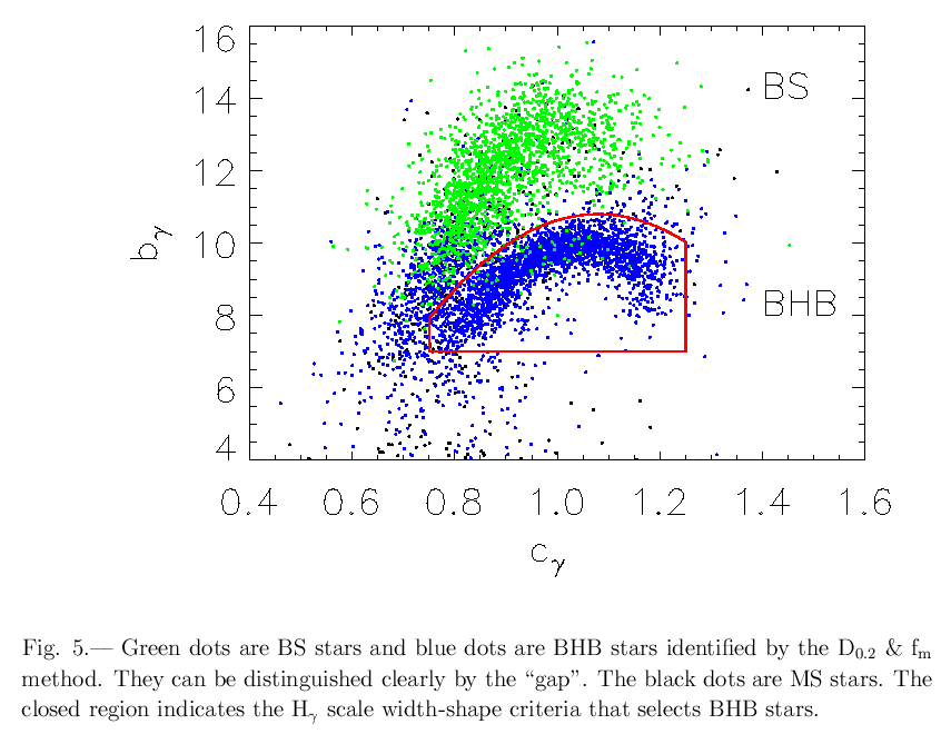
They end up with a sample of about 2500 BHB stars, sampling the Milky Way above and below the disk.
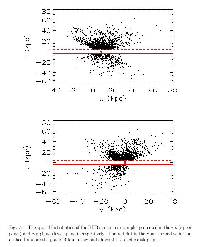
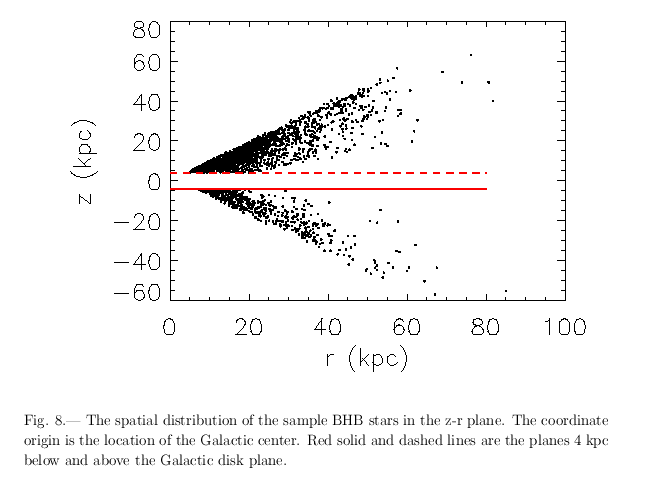
Now, each individual star provides only a limited amount of information compared to the VERA measurements of masers:
but
So, how can they derive the rotation curve from this information?
The answer is to create various self-consistent models of the Milky Way in a computer, and then sample these models in just the same way that the SDSS samples the real Milky Way. By picking models which match the SDSS measurements, one can get some idea for the Milky Way's actual properties.
The authors pick two SPH models, by Naab and Steinmetz. The models allow one to examine all sorts of properties of objects in the Galaxy, many of which we can't observe directly.
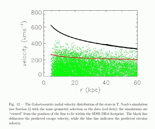
The authors then divide the real measurements, and the fake measurements, into radial bins, and compare the properties of objects in these bins. For example, they compute FROM THE MODEL the ratio
       V [line-of-sight]
       ------------------
        V [circular(r)]
Then, they find the model which best matches OBSERVED line-of-sight velocities. Finally, they scale THE OBSERVED line-of-sight velocities by the model's ratio to find the circular velocity at that radial distance.
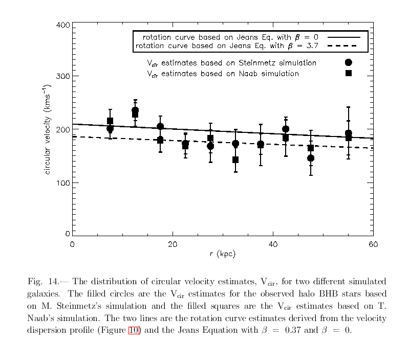
One can then fit arbitrary models to try to reproduce the deduced circular velocity as a function of distance.
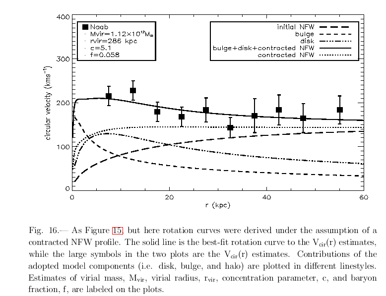
Note the size of the error bars in these measurements: about +/- 40 km/sec. The VERA result provided the circular velocity of one source to roughly 3 percent, or +/- 6 km/sec.