 Copyright © Michael Richmond.
This work is licensed under a Creative Commons License.
Copyright © Michael Richmond.
This work is licensed under a Creative Commons License.
Today marks the first day in which we will examine the cosmological distance ladder. Astronomers use many different techniques to measure the distance to celestial objects. Some are very reliable, based on geometry --- but only work for relatively nearby sources. Others can be applied to very distant sources --- but are much more indirect. One might compare the different techniques to a ladder, with strong rungs near the bottom, but shaky rungs at the top.
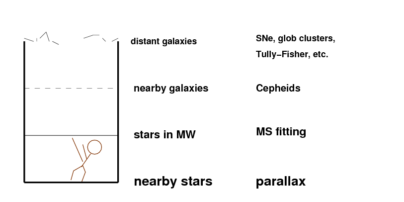
Today, we'll look at the bottom rung, focusing on techniques which are theoretically very sound, since they rely on little more than geometry. As we will see, however, these techniques are limited to stars and clouds of gas which are relatively close to the Sun; only one variant might possibly be applied to stars in the Magellanic Clouds.
Parallax uses the orbit of the Earth around the Sun to provide a baseline for measuring the angular shift of nearby stars against more distant ones.

The baseline d is in the simplest case the distance between the Earth and the Sun, 1 AU = 1.496 x 10¹¹ meters. If the star in question does not lie in the plane of the Earth's orbit, we must make a correction for the projection effects. The parallax angle π is defined as half the total shift, and is usually measured in units of arcseconds.
  Q:  Write a rigorously correct formula for the
      distance L to a star, if we have measured
      a parallax angle of π.


  Q:  Now write a simpler version which will be
      good enough for practical purposes.


  Q:  Why do astronomers prefer to measure distances
      in parcsecs instead of in meters?
Typical earth-based parallax measurements made with single optical telescopes can provide precisions of around +/- 0.03 arcsec. The best earth-based optical parallaxes can do about one order of magnitude better, with a precision of perhaps +/- 0.003 arcsec. So, how far out can we apply this method?
Let's begin with an analogy. Suppose that we want to measure the speed of a bird as it flies through the air. We use a meterstick to measure the distance it travels during an interval of t = 3 seconds. We measure a distance of x = 24 +/- 2 meters.
  Q:  What is the uncertainty in the
      measurement of distance?
      Express as a percentage.


  Q:  What is the speed of the bird?


  Q:  What is the uncertainty in the speed,
      expressed as a percentage?
That seems pretty straightforward. The uncertainty in the speed, in percentage terms, is the same as the uncertainty in the measurement of distance.
Let's try a parallax example. You look at the star Quizzle and measure a parallax angle of π = 0.12, with an uncertainty of
  Q:  What is the uncertainty in the
      measurement of angle?
      Express as a percentage.


  Q:  What is the distance to Quizzle?


  Q:  What is the uncertainty in the distance,
      expressed as a percentage?
Whoops. Because the measurement with uncertainty goes into the denominator of an equation, deriving the uncertainty in the derived distance is not so easy. Consider the common case of parallaxes which are have uncertainties which are larger than the measurement.

If you use a parallax measurement which has an uncertainty which is more than, say, one-tenth of the measurement itself, you should think carefully about the implications.
The most important catalog of stellar parallaxes was created by the Hipparcos satellite.
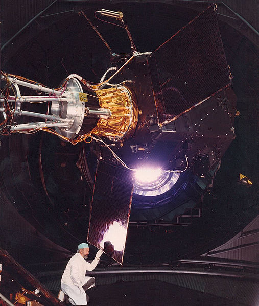
Image courtesy of
Michael Perryman
During the period from 1990 to 1993, Hipparcos measured the positions and brightnesses of roughly 2.5 million stars. The two main catalogs are

Image copyright
the European Space Agency.
There have been some minor changes to the Hipparcos results due to re-processing of the original data in the years since the first release of data, which was back in 1997. Be sure to check out van Leeuwen, A&A 474, 653 (2007) for details.
In the near future, we may expect to see a much larger catalog of stellar parallaxes from the GAIA satellite. This mission, currently scheduled for launch in 2012, will use an instrument which has the same basic design as the one in Hipparcos: a pair of telescopes, pointed in different directions separated by an angle of 106.5 degrees, which bring their light to a common focal plane, so that stars in one region of the sky can be compared to those in a different region of the sky very precisely. GAIA will be an improvement over Hipparcos in several ways.
Astronomers have attempted to measure parallaxes of stars using optical telescopes for hundreds of years (see Parallax: The Race to Measure the Cosmos for a good history). In recent years, however, some astronomers have found that radio telescopes can do a better job, at least in certain circumstances.
Stars emit most of their energy in the optical region of the spectrum, and very little in the radio; it isn't possible to detect most stars with radio telescopes. Clouds of gas and dust do emit plenty of radio waves, but they are for the most part large, extended sources, not the compact objects one requires for parallax measurements.
However, there are some circumstances which do allow radio astronomers to apply the power of interferometry to make very precise measurements of the positions of compact radio sources, and therefore to determine the distances to those sources via parallax. The key element is the maser emission from small clumps of gas within some star-forming regions. Astronomical masers arise within compact volumes, thus appearing as point sources to our radio telescopes, and produce radiation of very pure frequency. The combination allows astronomers to determine their positions with very small uncertainties.
There are several groups working in this area at the current time:
Let's focus on the VERA group. The instrument is a four-element interferometer,
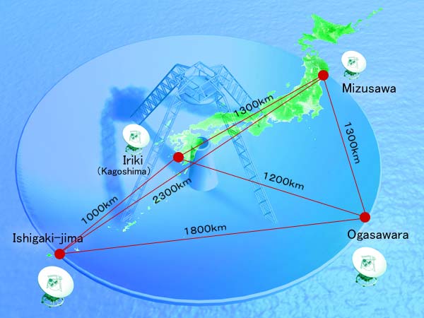
Image courtesy of
The VERA group and the National Astronomical Observatory of Japan
using dishes which are roughly 20 meters in diameter.
  Q:  What is the diffraction limit for an optical
      telescope like Hipparcos, which had a mirror
      of diameter d = 29 cm and measured light
      of wavelength λ = 500 nm?


  Q:  What is the diffraction limit for a radio
      interferometer like VERA, which has a typical
      spacing of d = 1300 km and measures
      radio waves from water masers at a frequency
      of f = 22.2 GHz?
If one looks at star-forming regions, such as S269, with an optical telescope, one sees clumps of stars immersed in gas and dust. If one looks with a radio interferometer, one can see much finer details. Compare the scales on the IR picture at left with the VERA map at lower right.
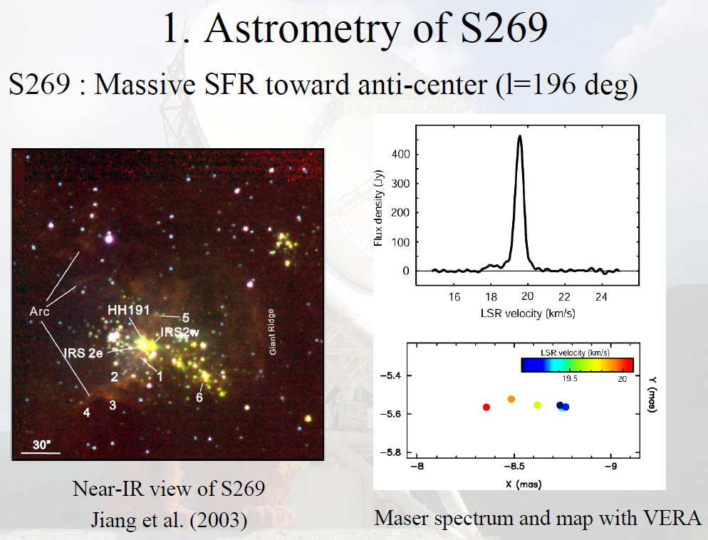
Image taken from
a presentation by Mareki Honma, NAOJ
If one measures the position of one of these masers over a period of several years, one will see an intriguing pattern. Shown below are VERA measurements of a maser in the Orion-KL region; the figure shows the Right Ascension component of the position as a function of time.
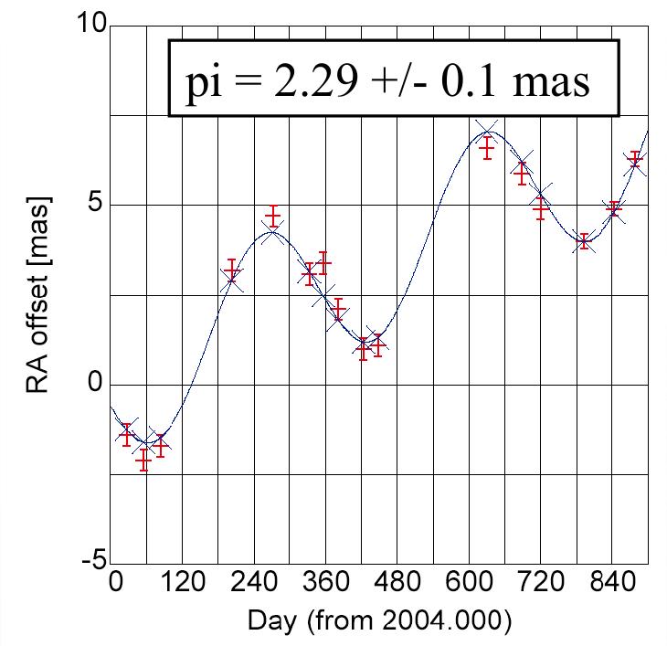
Figure taken from
a presentation by Mareki Honma, NAOJ ;
I've erased the parallax result so that my students can't
peek at it in class.
  Q:  What is the parallax to Orion KL
      based on the measurements above?


  Q:  What is the distance to Orion KL?
There are some situations in which we can't measure the distance to a single star of some particular spectral type directly because all the stars of that type are just too far away. In these situations, we can fall back upon two techniques which deal with groups of nearly identical stars:
The basic idea is each case is to select a sample of stars which are as identical as possible in spectral type and in apparent magnitude; that means that the all the stars in the sample ought to be at the same distance from us. Moreover, if we can collect a large enough sample of stars, we can assume (with only some small error) that the motions of the stars in the sample ought to be randomly distributed, so that the average motion over all stars relative to the Sun ought to be zero ....
.... except, of course, that the Sun is moving through the Milky Way with its own particular velocity. It is the reflection of that solar motion in the properties of this carefully chosen sample of stars that will tell us the distance to the stars in the sample.
We need to be precise. Since the stars in the disk of the Milky Way are all orbiting the center of the Galaxy with (approximately) equal speeds, and (approximately) in the same direction, we can define a local standard of rest: a circular orbit in the plane of the disk, with the average speed of all the stars at the Sun's distance from the Galactic Center. It is the Sun's motion relative to this local standard of rest that defines the solar motion. Determining the solar motion is a large task, all by itself, but let's take it as done for the current discussion.
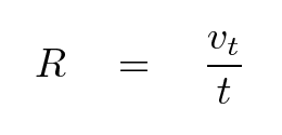
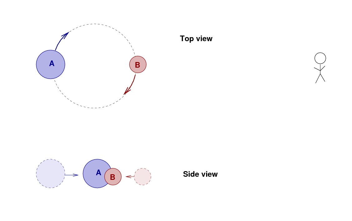
So, consider one of the many stars in this group, which is some unknown distance R from the Sun. Let's measure its proper motion t in the direction which is perpendicular to the Sun's motion through this spherical group. Because we've chosen to measure only the proper motion perpendicular to the Sun's motion, the speed of the Sun won't affect the value of t. All that matters is the star's own space motion in that direction, vt and the distance of the star R.


And so, if we knew vt and t for that star, we could compute the distance.
Alas, we don't know the value of vt for any star. Rats.
But we can say that if the stars in this sample are many, then the AVERAGE value of vt should be equal to the AVERAGE value of the radial velocities of the stars, which we can measure. Actually, that's not quite right. The star A in the diagram above is located directly to the side of the Sun, relative to the Sun's motion through space, so that the radial velcity of star A is not affected by the motion of the Sun v at all. But star B is a bit ahead of the Sun, so the radial velocity we measure for star B is a combination of the star's true motion away from the Sun's current location, rB, and the Sun's motion v. Look at the little inset at lower right -- we need to subtract the component of the Sun's v which is parallel to the star's motion rB.
But, once we have made that correction, we can use the (measureable) average radial velocities to stand in for the (unmeasureable) average tangential velocities, and thereby derive the distance R to the sample of stars.
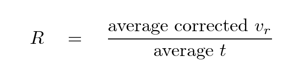
This method is known as statistical parallax.
  Q:  You measure the properties of a set of 68
      stars of spectral class K1.  Each star is
      roughly apparent magnitude m(V) = 12.3.
      The average proper motion of the stars in
      a direction perpendicular to the solar motion
      is 1.06 arcseconds per century.  The average
      corrected radial velocity is 6 km/sec.


      What is the distance to this set of stars?


      What is the absolute magnitude of a K1 star?
There is a very similar method which uses the components of proper motion which are parallel to the Sun's peculiar motion; it is called secular parallax. Secular parallax doesn't require the measurement of radial velocities, so it's a bit simpler in practice.
There's another technique which, like parallax, relies solely on very fundamental ideas. In this case, we're going to add a bit of very well-tested physics to the geometry, but I'd consider it still to be a rock-solid method for finding distances.
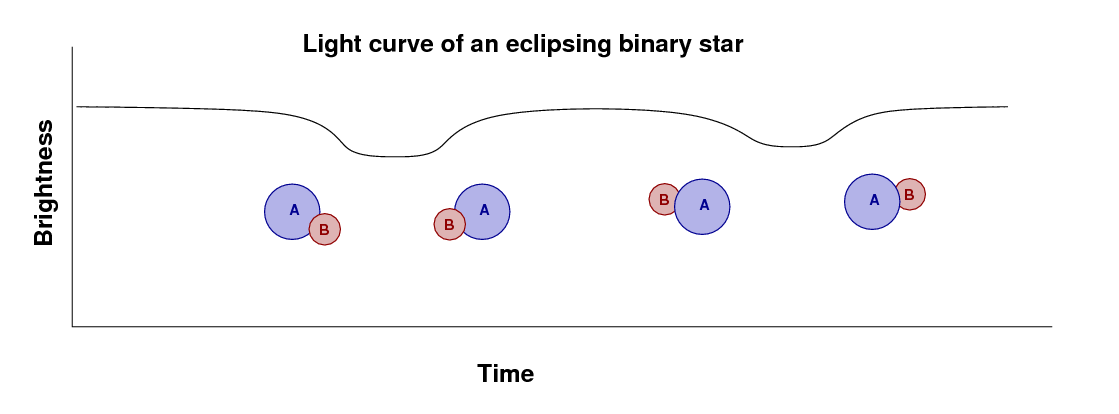
Suppose that two stars orbit each other in such a way that we see them pass in front of each other.
If we measure the light from the system over one full orbital period, then we'll see one dip in the brightness as star B passes in front of A, and then a second dip when A passes in front of B.
How can we use these binary stars to measure distances? We need to determine a number of parameters; we can divide the work into several steps.
Step II
Step III
The first step is pretty simple, and it doesn't involve a great deal of expertise. The second step is NOT simple, since stars do NOT emit like blackbodies at the level of accuracy which we need for this calculation. The third step is again pretty simple, though there can be complications due to extinction and reddening.
Let's go through just a few steps of this process in class. We'll use data from the paper The Distance to the Large Magellanic Cloud from the Eclipsing Binary HV 2274 .
Examine the figure below, which shows both radial velocities and the light curve of this binary as a function of time. The period of the system is 5.73 days.
Figure taken from
Guinan et al., ApJ 509, 21 (1998)
  Q:  What is the orbital speed of each star
      around the center of mass?
      You may pretend that the orbits are circular
      and equal in amplitude for this exercise.


  Q:  How long does the secondary eclipse at
      orbital phase 0.5 last?


  Q:  What is the size of each star?  You may
      pretend that the two stars are equal
      in size.
The authors go through the rest of the procedure and end up with a pretty good measurement of the distance to this system: 45.7 +/- 1.6 kpc. That's an uncertainty in distance of just about 3 percent!
However, the paper we've just discussed was published in 1998 and involves hot stars, for which stellar models may not be very accurate. A more recent study of eclipsing binary star systems in the LMC
uses binary systems with cooler stars, for which the stellar models are considered more accurate. Pietrzynski et al. (2013) claim that their set of 8 binary systems yields a distance to the LMC barycenter of 50.0 +/- 1.1 kpc, which is not quite consistent with the earlier results.
Copyright © Michael Richmond.
This work is licensed under a Creative Commons License.