 Copyright © Michael Richmond.
This work is licensed under a Creative Commons License.
Copyright © Michael Richmond.
This work is licensed under a Creative Commons License.
This discussion follows closely the version printed in An Introduction to Modern Astrophysics by Bradley W. Carroll and Dale A. Ostlie, in Chapter 27. Schneider's book covers the same ideas in Section 4.2.
The two questions we'll address today are:
We'll follow a simplified version of cosmology, one in which the cosmological constant is assumed to be zero. I find it easier to understand complicated ideas if I start with a simple case and add complexity later ...
Imagine that the universe is homogeneous and uniform, filled with matter which has the same density everywhere. Let's write the density of material as ρ(t), so at the current time, it has value ρ(t0), Consider a spherical shell of material of radius r, which is currently expanding at velocity v.
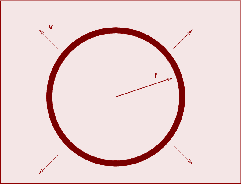
What will happen to the shell as time progresses?
The answer isn't too hard to figure out. One can make a close analogy to the motion of a cannonball which is fired vertically upward from the Earth's surface. There are two possibilities from a practical standpoint, or three if one is a mathematician.
The same is true for this shell of material. Let us demonstrate.
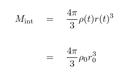
Because the universe is uniform, the gravitational forces from all the material OUTSIDE the shell cancel each other. That means that the dynamics of the shell depend only on the total mass enclosed by it. We will assume that the peculiar motions of matter are so small, compared to the large-scale motion of the shell as a whole, that the interior mass doesn't change as the shell expands.
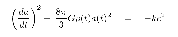
The shell itself has some mass m. We can write the total energy of the shell as a sum of its kinetic and gravitational potential energies. For reasons which will become clear later, I'll write that total energy in one particular manner.
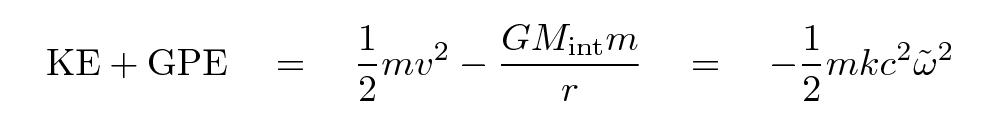
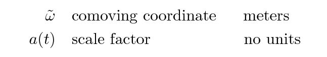
Now, as mentioned in the previous lecture, astronomers break the distance to an object into a portion which doesn't change with expansion, called the "comoving coordinate" and denoted as an ω with a tilde over it, and a portion which does, called the "scale factor" and written as a(t). If we substitute
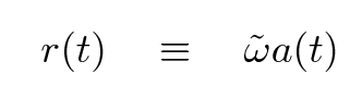
where
and do a little simplification, we end up with
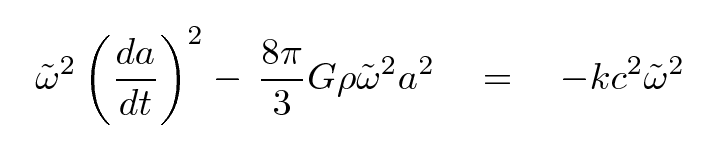
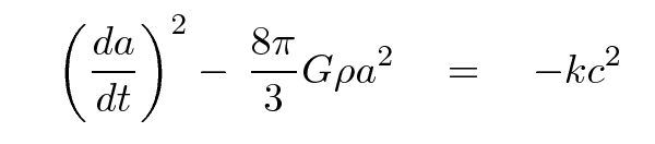
Let's stop for a moment and look at the result. The left-hand side shows the two terms which add up to form the total mechanical energy (per unit mass) of our shell of matter, and so the right-hand side must also be proportional to that energy. What are the possibilities?
It certainly would be nice to figure out the fate of our universe. Let's see if there is some way to convert that expression into one which contains observable quantities.
You may recall from the previous lecture that the Hubble parameter H(t) is related to the scale factor a(t) and its rate of change.
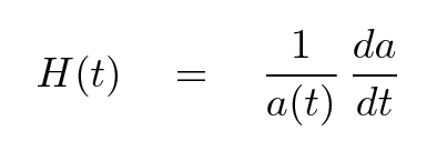
If we substitute this expression into our previous "energy equation", we end up with
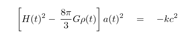
Now, this equation is valid for any choice of time. Note that the right-hand side isn't changing at all -- all the action is in the terms on the left. If we can measure some values which appear on the left hand side at ANY choice of time, we can compute the value of the right hand side once and for all. That, in turn, will tell us the fate of the universe.
So, what's a good time to choose? How about .... RIGHT NOW! I'll use a shorthand for t = now by placing a zero subscript on quantities; that turns H(t) into H0, which may look familiar to you.
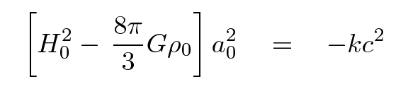
  Q:  What is the value of H0?


  Q:  What is the value of a0?


  Q:  Can you compute the value of the
      critical density of the universe at
      the current time?
The critical density is an important value, but if one specifies it in grams per cc or kg per meter cubed or atoms per cubic meter, it always seems to involve a large negative exponent. For convenience, cosmologists often discuss the matter density in a relative way:
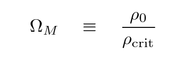
The "M" subscript refers to all matter, ordinary baryonic and exotic dark matter alike.
What is the value of ΩM? There are many ways to measure it ..
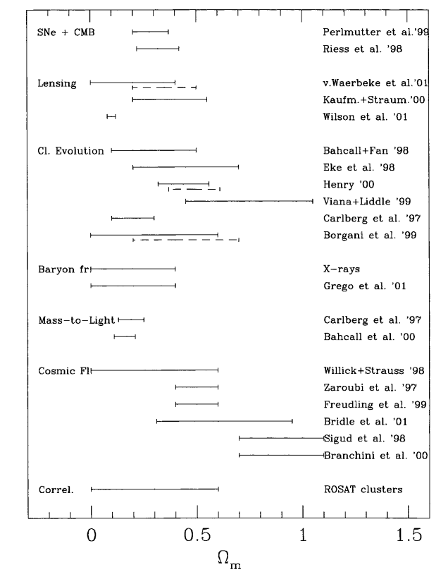
Figure taken from
Schindler, SSRv 100, 299 (2002)
.... but the conclusion is pretty clear: it's not close to the critical value. That means that if the universe is as simple as we've assumed, it will expand forever.
Okay, so we have a good qualitative notion for the future of our (overly simplified) universe; can we make it more quantitative? We know how fast the universe is expanding here and now, and we have some measures of the density of matter; that means we ought to be able to compute the future rate of expansion and size of the universe, right?
Right. Let's go back to an earlier version of the "energy equation" for a shell of matter in the uniform universe.
The density of matter does change with time, and the scale factor does change with time ... but the total amount of matter inside the shell does NOT change with time.
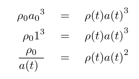
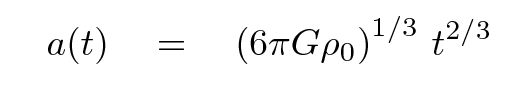
We can use this relationship to create a differential equation for the scale factor as a function of time.
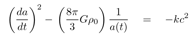
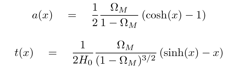
Well, there it is: a differential equation for the scale factor and its first derivative. We know the value of the scale factor now, and the value for the rate of change now, so, in theory, we ought to be able to compute the value of the scale factor for any arbitrary time in the future or the past. Sure, we may not know exactly what the value of the constant on the right-hand side is, but we can figure out the result for each of the possibilities.
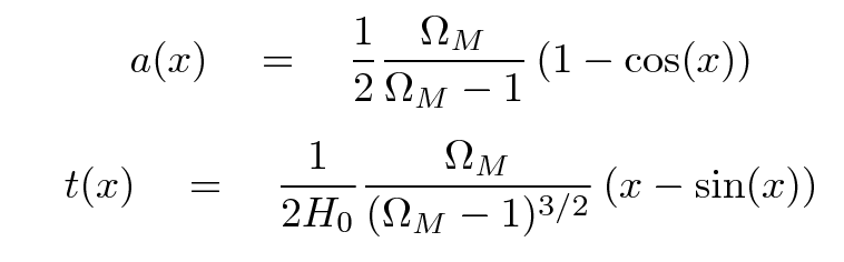
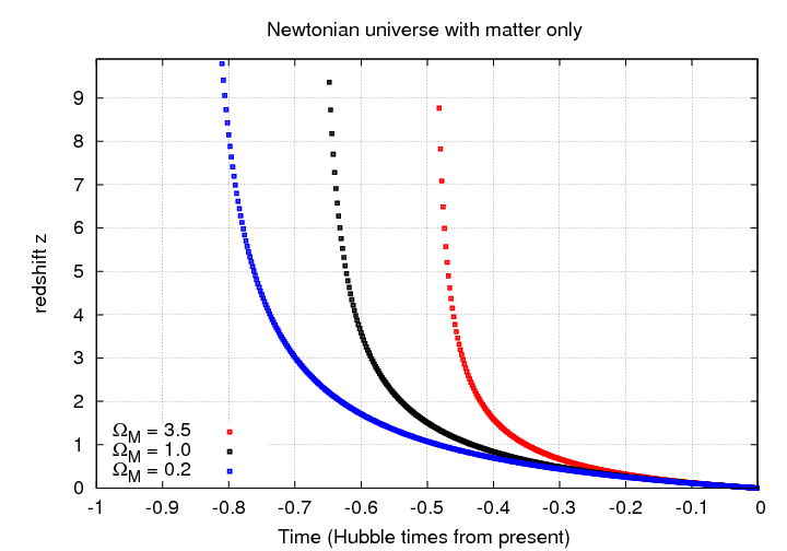
Below is a graph showing the evolution of the scale factor as a function of time for three choices of ΩM. On the horizontal axis is time, but the units aren't seconds or years or gigayears; instead, they are in "Hubble time" units. One "Hubble time" is simply the reciprocal of the current value of the Hubble parameter. For rough purposes, one call say that one Hubble time is about 10 Gyr, for the current universe in which we live.
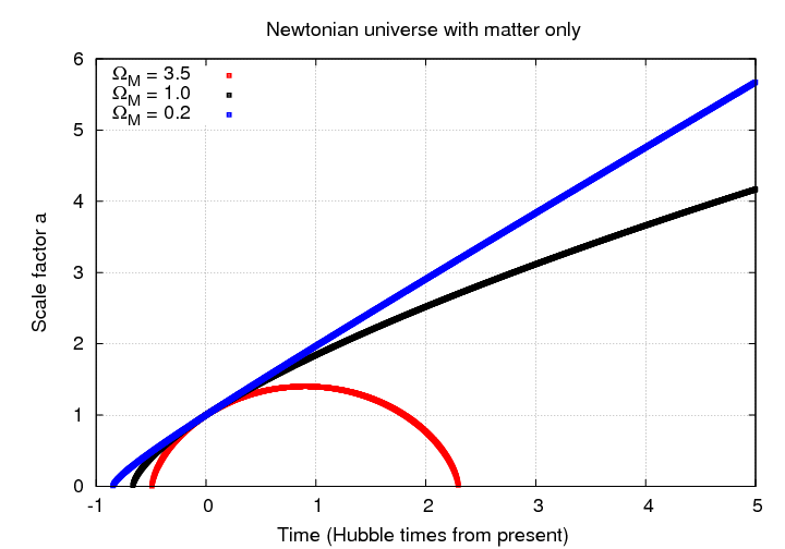
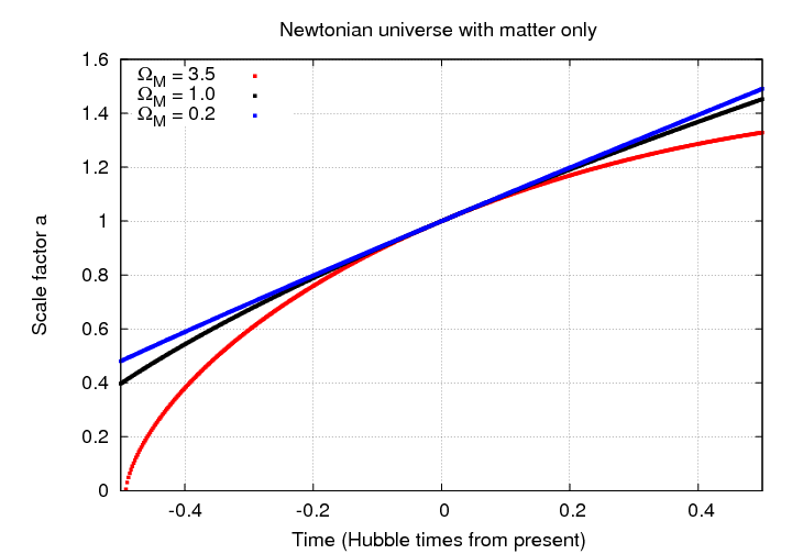
Even though each universe has a very different scale factor in the far future, it isn't so easy to distinguish them either in the near future, or -- more important -- in the near past.
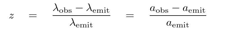
So, we have a way to describe the scale factor as a function of time. That's fine, but it doesn't really help observational astronomers. When we take images and spectra of distant objects, we don't get a timestamp telling us when the light was emitted. However, we DO get one piece of information which tells us something equivalent to time: the redshift z.
The redshift is usually expressed in terms of the emitted and observed wavelengths of light, but it can just as well be written in terms of the scale factors at the time of emission and observation.
  Q:  Write an equation which expresses redshift
      z in terms of a, the scale
      factor at the time light was emitted.


  Q:  Write an equation which expresses the
      scale factor a at the time
      when light was emitted as a function
      of redshift z.
Since we have procedures for computing the scale factor as a function of time, we can use these relationships between redshift and scale factor to produce tables or graphs of redshift as a function of time.
The Hubble parameter is related to the rate at which the scale factor is changing with time; one might think of it as something like the "velocity" of the scale factor. It is sometimes handy to discuss the second derivative of the scale factor -- something like its "acceleration."
Cosmologists have adopted the deceleration parameter q as a measure of this property of the scale factor. It is defined formally as
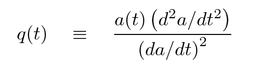
but for the simple universe we are considering today, which contains only matter (and no cosmological constant),
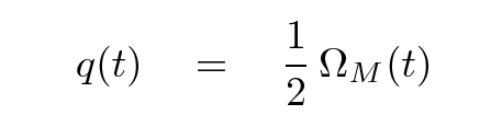
If we consider the value of this parameter at the current time, q0, we see (again) a cosmological parameter which can fall into three important domains:
We're finally ready to address the second question posed at the start of today's lecture:
We need to find a way to bring observable quantities -- such as magnitudes and redshifts -- into the discussion of scale factors. In order to do so, we'll start with the Robertson-Walker metric:
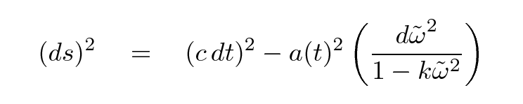
"What is this quantity ds," you ask? Well, in the simple case that space is flat (k = 0) and static (a(t) = 1), this expression for ds turns into the Space-Time Interval. That's the interval between two events, which will be the same as measured by any inertial observer. Confused? Try reading a bit from an introductory course on Special Relativity.
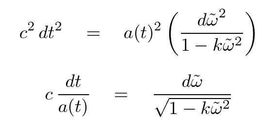
Since we'll be observing light rays which were emitted by objects long ago and far away, let's consider the motion of a light ray. The spacetime interval ds between the emission and absorption of the light ray will be zero, so
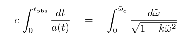
We can integrate both sides of this equation to find the proper distance ω between the emission (t = 0 and ω = ωe) and absorption (t = tobs and ω = 0) of the light ray.
Performing that integral will give us the proper distance as a function of TIME; but it would be much more useful to have an expression for proper distance as a function of REDSHIFT. Fortunately, we know how the redshift z is related to the scale factor a, and how the scale factor a is related to time, so it is possible to do the integral over redshift as well. Let's just skip to the result:
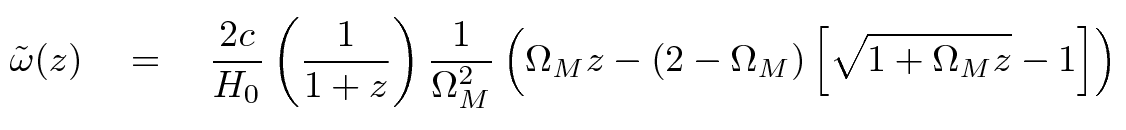
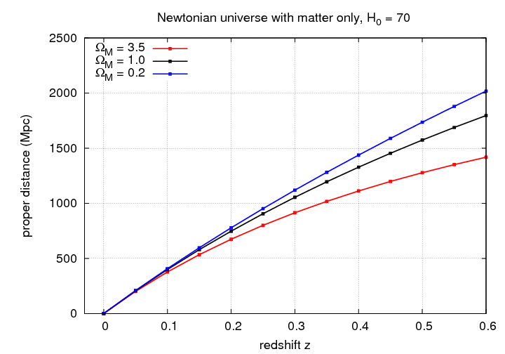
This is a complicated equation, but it can reduce to a pretty simple result. If one looks at very small redshifts, one finds that the distances for different cosmological models are all about the same, AND they all are linear with redshift.
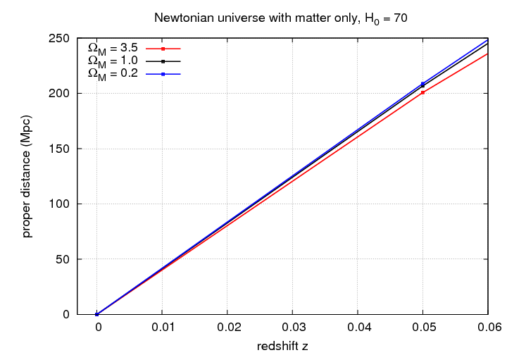
But at larger redshifts, the distances diverge from each other and from the simple linear relationship.
  Q:  For the case that k = 0,
      derive a simpler expression
      for proper distance as a function
      of redshift.
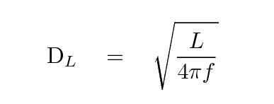
Do you remember the definition of luminosity distance?
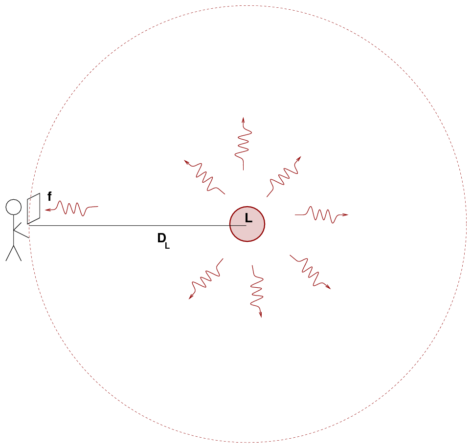
If we know the luminosity L of the source, and measure the flux f, then we can compute a distance using the inverse square law.
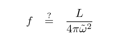
Since we now have a way to compute the proper distance to an object as a function of redshift, it might seem unnecessary to compute the luminosity distance: isn't it just the same as the proper distance? If so, then we could simply write:
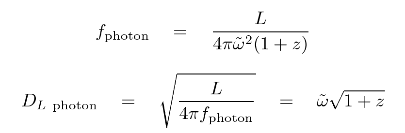
This causes photons to arrive at our detector less frequently by a factor of (1+z).
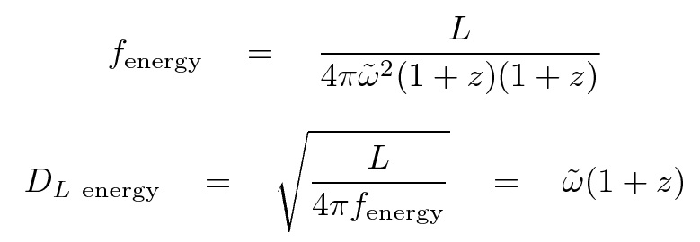
Since the wavelength of each photon is longer, the energy it carries is smaller: Eobs = Esource / (1+z) .
Depending on the sort of detector we use to measure light from a distant object, we'll find a flux which differs from the naive expectation by a different amount.
If we use a detector which counts photons, such as a CCD, then we will suffer from the time dilation factor; but if we properly account for the shift in the passband between the source and observer frames, we won't be affected by the decrease in energy of each photon. We can define a photon-based luminosity distance like so:
On the other hand, if we use a detector which converts the incoming flux of energy into an output signal, like a bolometer, then we are affected by both the time dilation and the decrease of each photon's energy. In this case -- which is the one described in most textbooks -- we can define a energy-based luminosity distance like so:
Once we have the proper expression for luminosity distance, we can use it to compute the distance modulus of an object at any particular redshift. That means we can finally begin to compare models of the universe with different cosmological parameters to actual observed quantities.
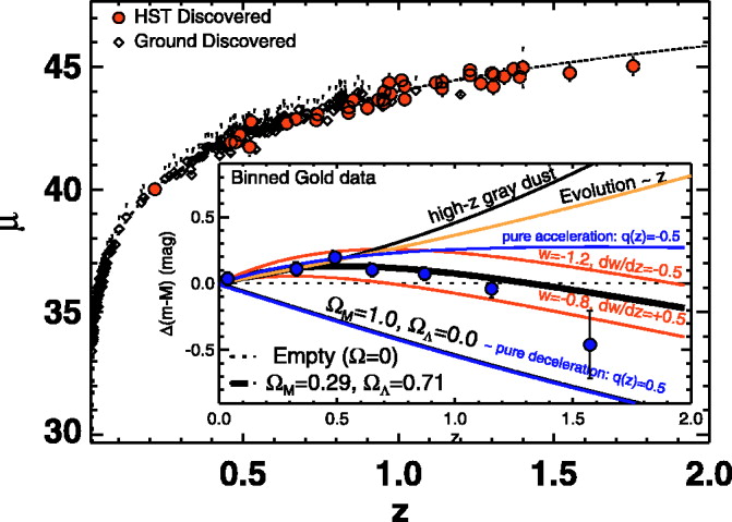
Figure taken from
Riess et al., ApJ 659, 98 (2007)
Copyright © Michael Richmond.
This work is licensed under a Creative Commons License.