 Copyright © Michael Richmond.
This work is licensed under a Creative Commons License.
Copyright © Michael Richmond.
This work is licensed under a Creative Commons License.
You all probably know about Mr. Hubble and the relationship he described between the recession velocity of galaxies and their distances. But you may not know how hard it was for him and the other astronomers of the time to determine the necessary data:
How did Hubble determine the distances to galaxies? As described in Hubble and Humason, ApJ 74, 43 (1931) , he used Cepheid variable stars when possible, since he recognized that they were the best of the available distance indicators; but he could measure their properties only in members of the Local Group, such as M31 and M33. For more distant galaxies, Hubble was forced to rely on indicators which he fully recognized were less accurate:
We know now that some of the objects which Hubble considered isolated stars were unresolved blends of star clusters or HII regions. Thus, many of his measurements of distances were underestimates, since he assigned the combined light of many stars to that of a single star.
Now, as for the second part of the required dataset -- radial velocities -- Hubble relied in large part on measurements made at Mount Wilson, which had the largest telescopes in the world at that time. Much of the work was done by Milton Humason, who rose from the position of mule driver and janitor to become one of the best observational astronomers of his day.
Many of the crucial spectra were taken with the 100-inch (2.5 meter) telescope at Mount Wilson. As an example, consider the spectrum of NGC 7619. Humason took two photographs:
During the past year two spectrograms of N. G. C. 7619 were obtained with Cassegrain spectrograph VI attached to the 100-inch telescope. This spectrograph has a 24-inch collimating lens, two prisms, and a 3-inch camera, and gives a dispersion of 183 Angstroms per millimeter at 4500. The exposure times for the spectrograms were 33[h] and 45[h], respectively.
Based on the two spectra, Humason estimated the velocity of NGC 7619 to be 3828 and 3754 km/s; he found a weighted average of 3779 +/- 100 km/s.
Below are samples of other spectra taken by Humason with the 100-inch telescope and similar equipment.
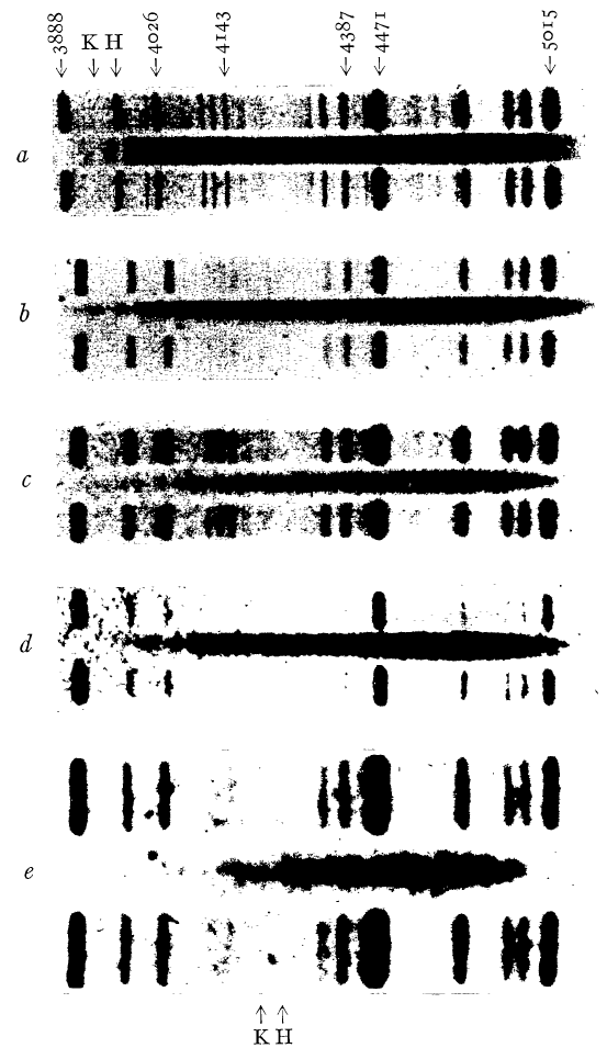
Figure taken from
Humason, ApJ 74, 35 (1931)
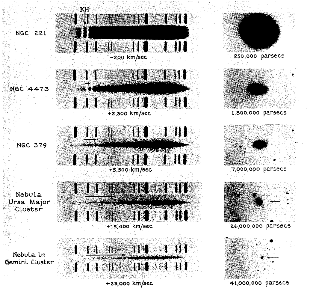
Figure taken from
Humason, ApJ 83, 10 (1936)
Astronomers in recent years have also measured the velocity of this galaxy. Wegner et al., AJ 126, 2268 (2003) used a telescope of similar size, the MDM 2.4 m at Kitt Peak, to acquire a spectrum with roughly the same dispersion, about 140 Angstroms per mm. However, the modern spectrum
So, give it a try: use the original Hubble diagram to measure the relationship between velocity and distance.
Figure taken from
Hubble, PNAS 15, 168 (1929)
Okay, fine: so there's a linear relationship between the distance to a galaxy and its recession velocity. What does any of that have to do with expansion?

Mathematically, this behavior can be described by breaking the ordinary concept of "distance" into two pieces:
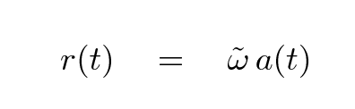
The radial velocity of an object is simply the time derivative of its distance from us,
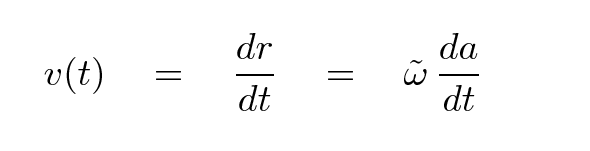
Now, an observational astronomer like Hubble might choose to describe the radial velocity of a galaxy in a different mathematical manner, like this:
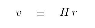
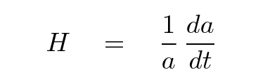
  Q:  Combine these two ways of describing velocity
      to find an expression for the Hubble constant
      H in terms of the scale factor a(t).
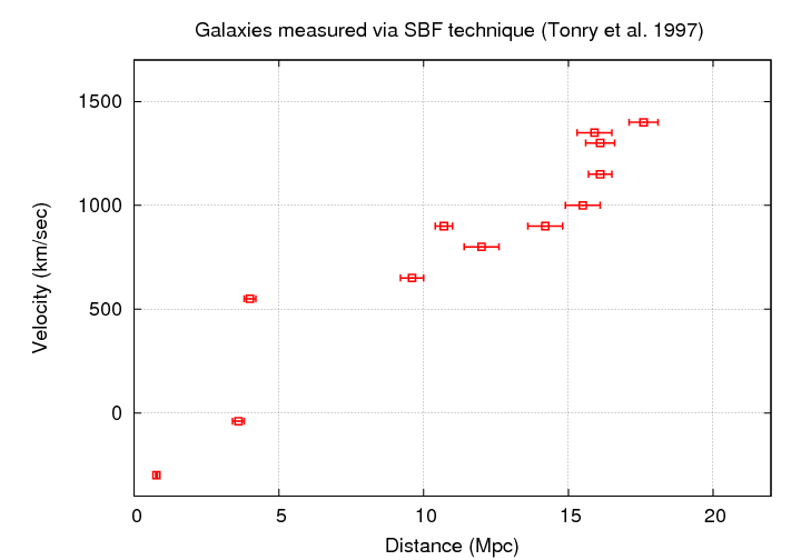
We now rely on other means to measure distances to nearby galaxies: in addition to Cepheids -- which we can detect in much more distant galaxies than Hubble could -- we use SBF, PNLF, TRGB, GCLF. Below is a graph showing the distances measured using the SBF technique (Tonry et al., ApJ 475, 399, 1997) to a set of galaxies which is similar to that used by Hubble. The velocities are very similar, but the distances are not.
Take another look at the value of the Hubble constant:
If we take the reciprocal of this expression, we end up with
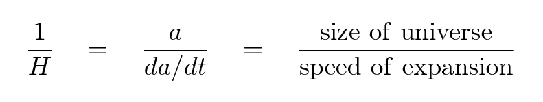
If we pretend that the expansion of the universe has been constant, which will turn out not to be a terrible assumption, then we can compute the age of the universe simply by taking the reciprocal of the Hubble constant.
  Q:  Adopt a value of H = 70 km/sec/Mpc.

      Convert the value of H to units of 1/seconds.
      What is it in those units?


      What is the age of the universe based on this
      value of H?
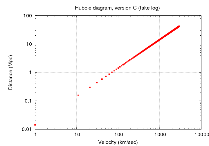
The original "Hubble Diagram" placed distance on the vertical axis and recession velocity on the horizontal axis. In that diagram, a uniformly expanding universe -- when measured over small distances -- produces a straight line.
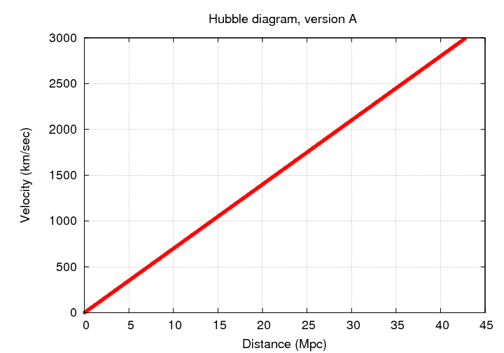
However, there are many other graphs you will see in the astronomical literature which also go by the name of "Hubble diagram". All of them show some aspect of the relationship between distance and recessing velocity, but involve different ways to express these two quantities.
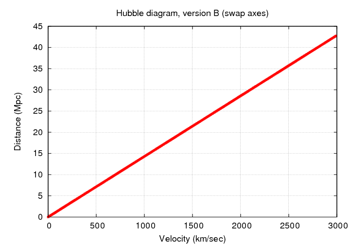
First of all, most of the diagrams swap the axes, so that a velocity-like quantity is on the horizontal axis and a distance-like quantity is one the vertical axis.
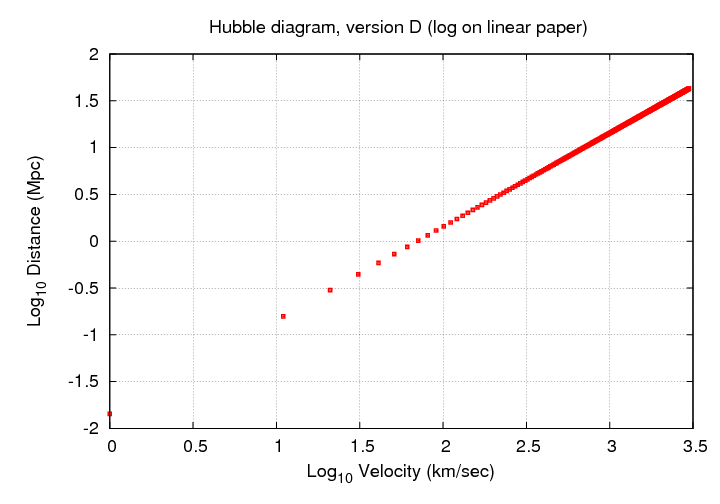
Once we move far beyond the Local Group, it often becomes convenient to switch to some sort of logarithmic scaling, so that all the points will fit on the graph without a big pile in the lower-left corner.
Remember this figure, for example?
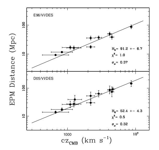
Figure taken from
Jones and Hamuy, RMxAC 35, 310 (2009)
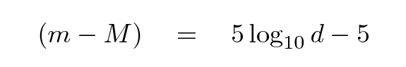
Instead of measuring distance in Mpc, astronomers sometimes choose to express distance in terms of the distance modulus
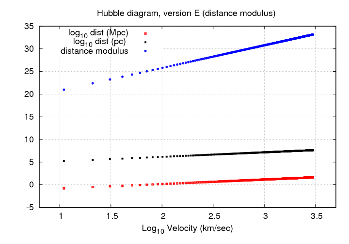
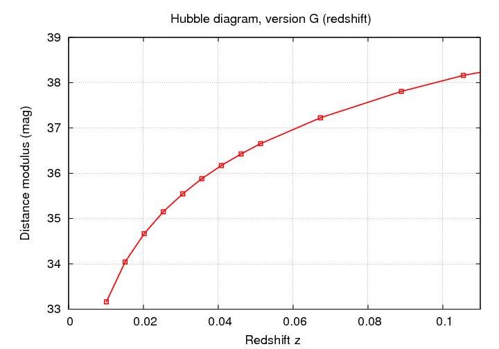
So far, every diagram we've made shows a linear relationship. Alas, all good things must come to an end. If we measure galaxies which are really far away, redshift becomes the convenient observational quantity. Now, at low redshift (z < 0.1), there's a simple relationship between velocity and redshift:
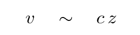
A Hubble diagram of distance modulus against velocity shows a curved locus for objects which flow freely in expanding space,
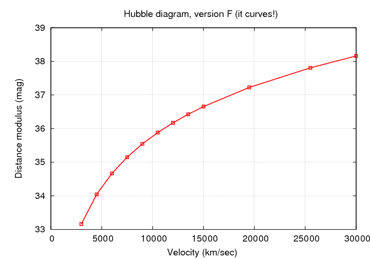
and therefore, so does a diagram showing distance modulus against redshift.
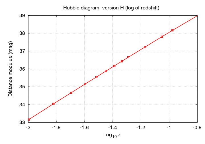
However, if we compute the logarithm of the velocity,
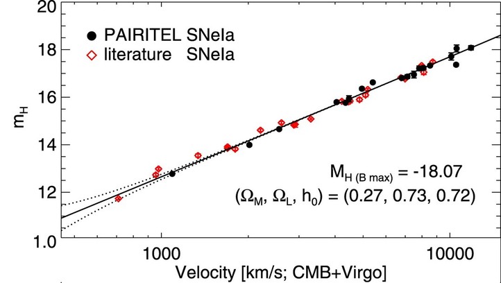
Figure taken from
Wood-Vasey et al., ApJ 689, 377 (2008)
and slightly modified.
or the logarithm of the redshift, then we once again see a nice, linear relationship.
You should be ready to convert from any set of units to an equivalent set of units, and to understand whether the slope of some particular "Hubble diagram" is simply related to the Hubble constant or not.
Note that all the examples in this section have considered only galaxies which are close enough to the Milky Way that their recession velocities are much less than the speed of light; another way to say that is that the redshifts are all less than one. As long as we stay within this small region, we can expect the simple relationship discovered by Hubble to be accurate.
When astronomers begin to cast their gaze into the distant reaches of space, where the redshift due to cosmological expansion starts to grow beyond a few percent, they encounter a problem. How can one fairly compare the measurements of galaxies near and far when the portion of a galaxy's spectrum which is sampled by a given passband changes?
Consider an ordinary spiral galaxy at redshift zero. We can express the flux of energy emitted by the galaxy as a function of wavelength in some form like this ("flam" as opposed to "fnu"):
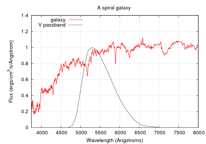
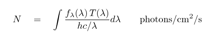
We can compute the number of photons which enter our detector by convolving the spectrum fλ with the passband T of the detector.
If we observe an identical galaxy at z = 0.05, we will find that this small dip in the spectrum moves into the most sensitive region of the passband.
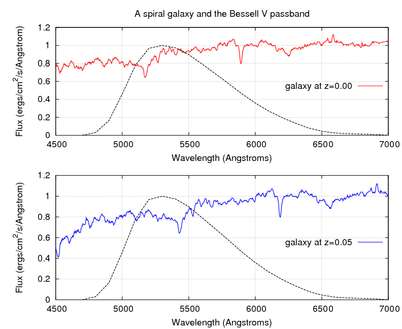
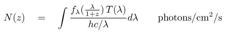
As a result, the number of photons which enter our detector will be slightly smaller than we would expect. Mathematically speaking, the number of photons we detect is now the convolution of the passband with the redshifted spectrum.
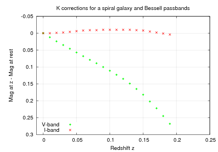
The difference increases with redshift, as the photon-poor UV region of the spectrum shifts into the V passband.
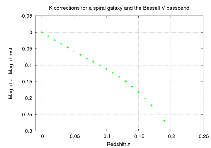
Astronomers who compare nearby galaxies to distant galaxies must account for this change in apparent magnitude in addition to the decrease in brightness due to distance via what we call K corrections.
Note that the effect of the redshift depends on both the shape of the spectrum and on the choice of passband. Suppose we observe the same spiral galaxy through the Bessell I passband.
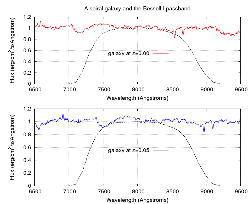
  Q:  Estimate the K correction for this galaxy
      at z = 0.05.   Will the galaxy appear
      brighter than expected or fainter than expected?


      Is the K correction for the I-band larger or
      smaller in size than the K correction for
      the V-band?
The K corrections depend strongly on the shape of the galaxy's spectrum. Spectra with relatively sharp changes are likely to yield large K corrections. Elliptical galaxies, with their lack of hot, young stars, produce very little light in the blue and near-UV; as a result, they have large K corrections in the B-band.
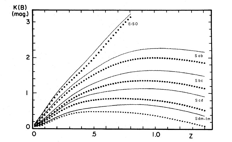
Figure taken from
Pence, ApJ 203, 39 (1976)
The dotted lines include corrections for
extinction within the Milky Way.
When one studies objects at redshifts beyond z = 0.1 or so, one finds a curious but perhaps useful fact: the region of the spectrum sampled at zero redshift in one of the typical wide-band astronomical filters -- say, the B-band -- is not so different from the region of the spectrum of an identical object at high redshift, measured through a different filter -- say, the V-band.
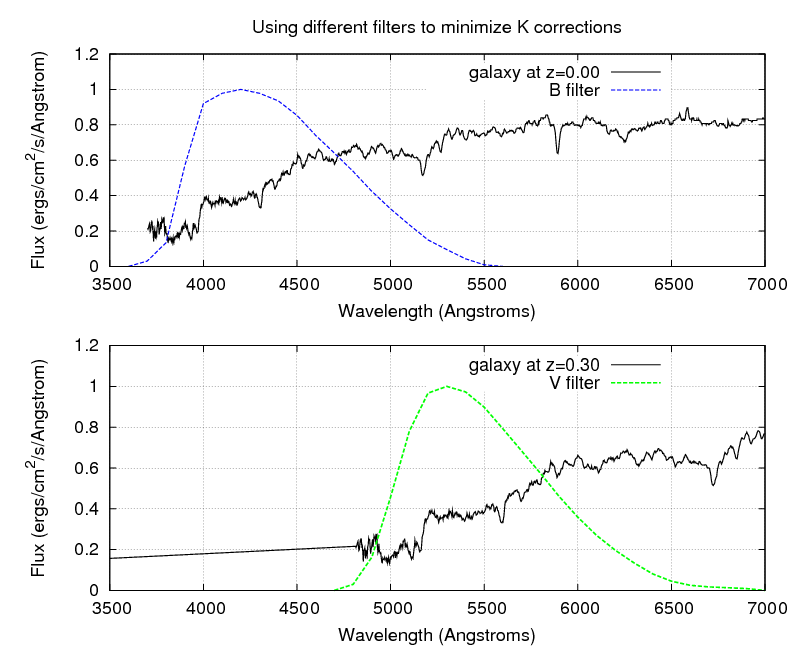
Some astronomers who study Type Ia supernovae, such as Kim, Goobar and Perlmutter, PASP 108, 190 (1996) , use different filters when they measure supernovae at different redshifts, in order to decrease the size of the K corrections they need to make. Note that this approach will only work if one's model for the spectrum of the object in question is accurate AND if the objects at different redshift really are identical.
In ordinary life, the concept of "distance" is obvious: it describes the separation between two objects. Whether one uses a meterstick, a string, a laser beam, or any other device, one will end up with the same result. The method doesn't matter.
In the "nearby" universe, the Local Group and nearest big galaxy clusters, the same is true. But when we study objects at redshifts beyond a few percent, we discover that the method DOES matter. Therefore, before we start looking at galaxies and quasars in the distant universe, let's define a few terms.
Let's consider these methods in turn. The angular-diameter distance to an object of linear size s depends on the angle θ it subtends.
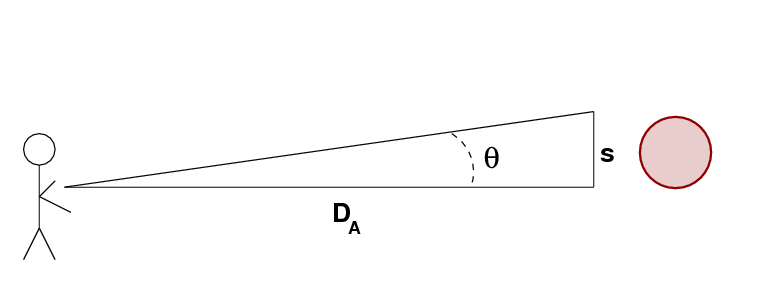
  Q:  Write a formula which yields DA
      as a function of the other quantities.

  Q:  The planet Jupiter is known to have an equatorial
      radius of R = 71,500 km.  On the night of Tuesday,
      May 3, 2011, the angular diameter of the planet
      is measured to be 33.5 arcseconds.


      What is the angular diameter distance to Jupiter?


  Q:  If we were to observe Jupiter from larger and larger
      distances, how would its apparent angular diameter
      change?
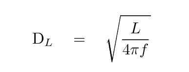
The luminosity distance, on the other hand, is defined by the relationship between the amount of energy the object radiates L and the flux of energy f we observe through some specified area.
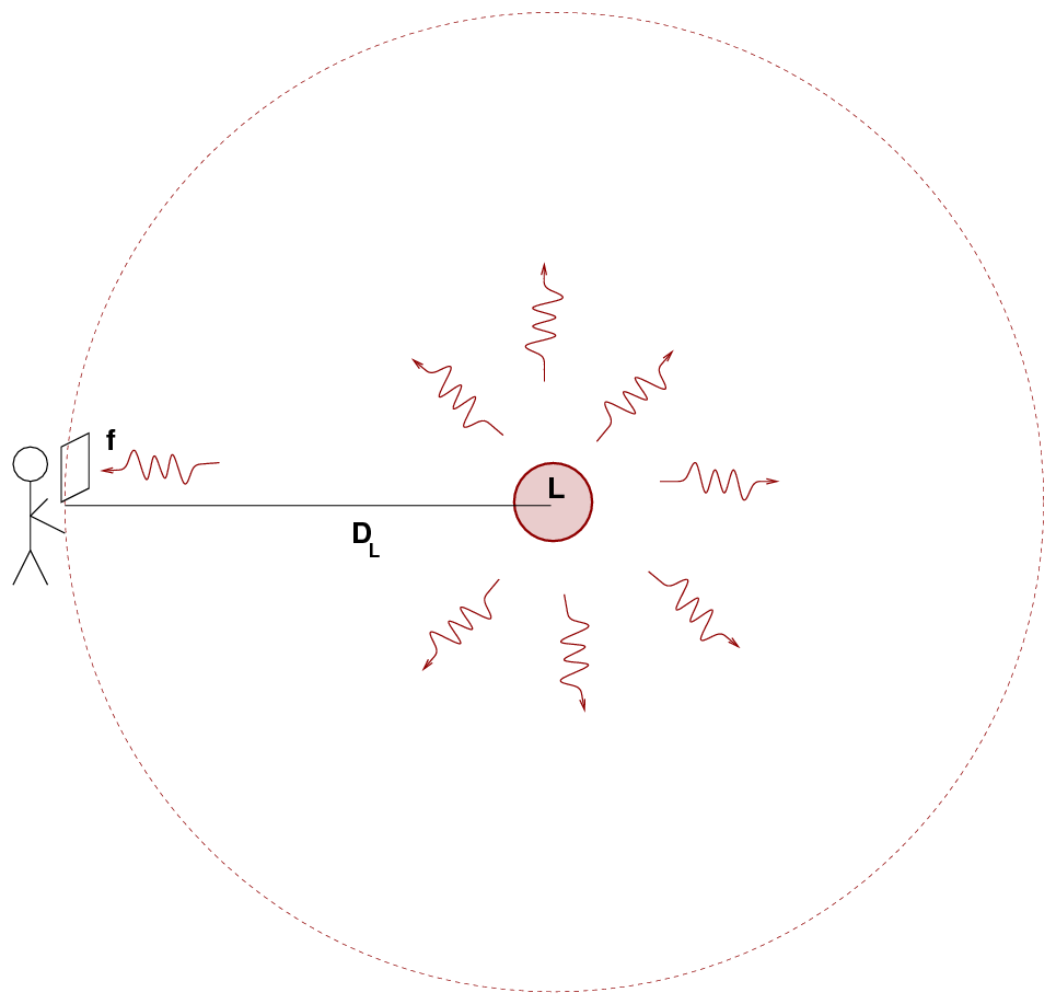
  Q:  Write a formula which yields DL
      as a function of the other quantities.
  Q:  The planet Jupiter is known to have an infrared
      luminosity of L = 2.85 x 10¹⁹ Watts.
      On the night of Tuesday, May 3, 2011, the infrared
      flux from Jupiter is measured to be
      2.93 x 10⁻⁶ Watts per square meter.


      What is the luminosity distance to Jupiter?


  Q:  If we were to observe Jupiter from larger and larger
      distances, how would its luminosity change?
Copyright © Michael Richmond.
This work is licensed under a Creative Commons License.