 Copyright © Michael Richmond.
This work is licensed under a Creative Commons License.
Copyright © Michael Richmond.
This work is licensed under a Creative Commons License.
Last time, I discussed the absorption of light in the infrared by carbon dioxide, due to transitions from the ground state to the vibrational modes. I showed -- briefly -- this figure.
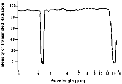
Figure 5 taken from
Infrared Spectroscopy
a part of
Yun Hee Jang's General Chemistry class
at CalTech.
"But what about the big dip at about 14 microns?" asked Mr. Monteleone.
Well, today, I can tell you just a little bit about that feature.
The oscillations we discussed last time involved the motions of oxygen atoms toward and away from the central carbon atom in a CO2 molecule. If you watched one molecule oscillate over time, it would look something like this:

Note that all the motions are in a straight line. Physicists call this the stretching mode.
It turns out that the molecule can oscillate in other ways, too. For example, the atoms can move in a plane which lies perpendicular to the line connecting the atoms; in other words, the atoms might move "up" and "down" over time, like this:

This sort of motion is called the bending mode of the molecule. Evidently, the strength of the bonds between the atoms in this direction is somewhat weaker than it is to radial (in-and-out) motions. I've tried to find some explanation for the difference in the effective spring constant, but failed. Sorry.
The important point is that when the molecule oscillates in this bending mode, its energy is lower than in the stretching mode. So, a transition from the ground state to this excited "bending-mode" state requires less energy than one to the "stretching-mode" state. Less energy means a lower-energy photon is absorbed, which means a longer wavelength.
Here, for example, is a graph showing the absorption spectrum of CO2 in the near-infrared. The "stretching-mode" and "bending-mode" transitions can be seen more clearly. The units on the top scale are microns. (Scroll to right to see the entire spectrum)
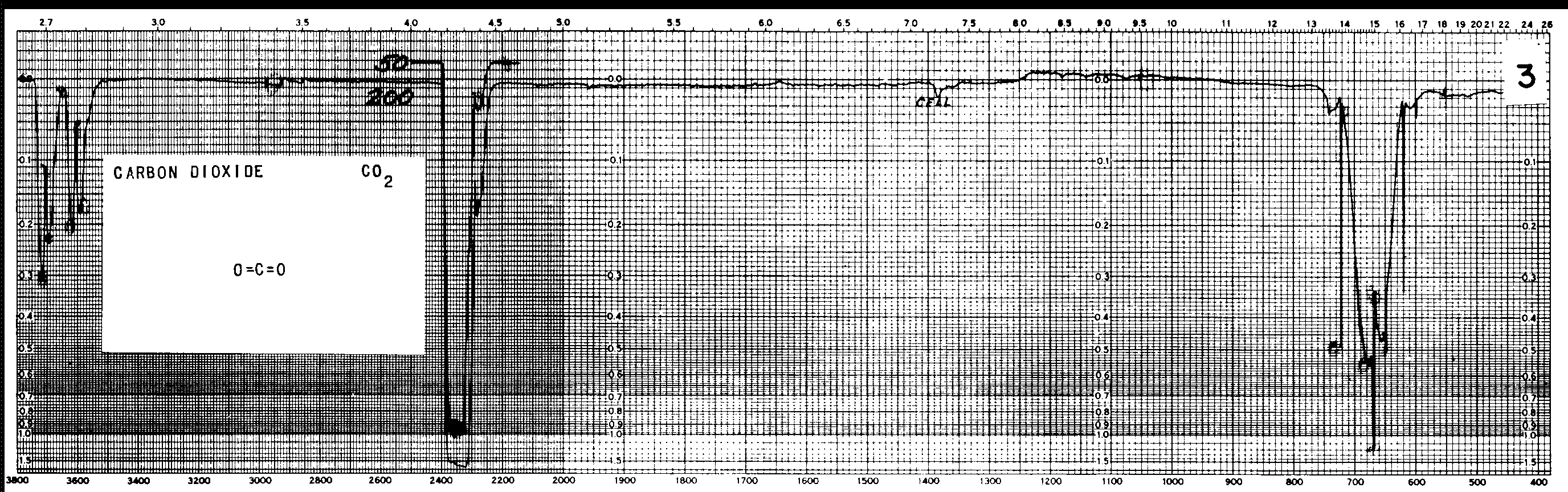
Figure taken from
NIST Chemistry WebBook, SRD 69
But things are much more complicated if one looks in detail. The figure below shows a closeup of the 15-micron, bending-mode absorption feature. It's not a single line -- it's a veritable forest. There are lots of smaller energy levels hidden within this bending mode.
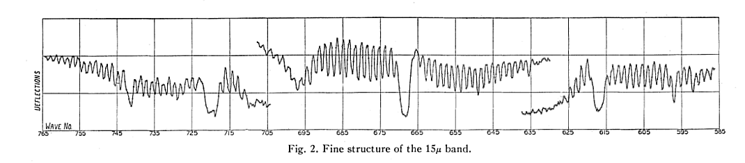
Figure 2 taken from
Martin and Barker, PhysRev 41, 291 (1932)
Molecular spectroscopy is a very powerful tool for investigating the properties of a gas, but it's also a complicated subject.
In the second week of this class, we learned how to handle a simple oscillator which suffers from damping. In recent weeks, we learned how to analyze the behavior of coupled oscillators. So, can we combine this information, and figure out how to model the motion of a pair of oscillators which each experience a damping force?
Let's try!
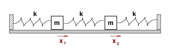
We'll start with a basic setup: two identical blocks, each of mass m, which are joined to fixed walls, and to each other, by identical springs with force constant k.
But now, add a new ingredient: each block suffers from air resistance, with a force directed opposite to its motion, and with a size linearly related to its velocity. In other words, a resistive force
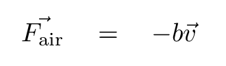
Our analysis begins in the usual way: we write down the forces on each block, and I give up on the vector signs :-/

The next step is to replace the expressions for force and velocity with those involving derivatives of the positions of the blocks with respect to time.

Now, at this point, we can take several different paths toward a solution. Remember this pair of equations in a red box, because we'll come back to it later.
For now, we'll take the same simple approach that we used in our first encounter with coupled oscillators.
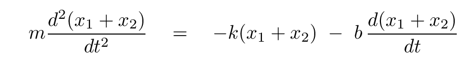
Q: What happens if one adds these two equations together?
Once we re-arrange things a bit, we end up with
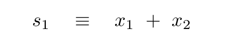
This looks suspiciously familiar, doesn't it? Suppose we define some new variable
Then this becomes
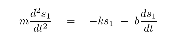
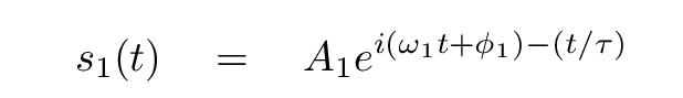
Aha! We know how to solve THAT equation, for a single variable. The solution is a damped harmonic oscillator. We can write it as a cosine multipled by a negative exponential
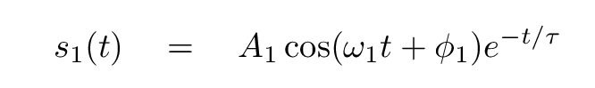
or as a complex exponential (of which the position will be the real part).
  Q:  How can we find the values of the frequency ω1
           and the time constant τ?
All we have to do is to plug one of these expressions for s1(t) into the differential equation, and force both sides of the equation to equal each other.
The work is a bit simpler if we choose the exponential form. In that case, the derivatives are
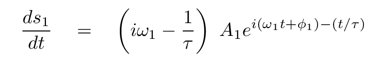
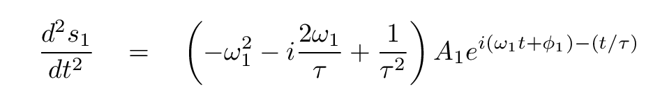
So, if we substitute the above expressions for the derivatives into the differential equation
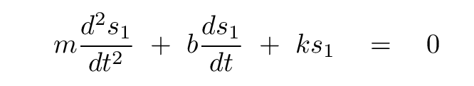
we end up with three terms. Each term has a factor of A1 times an exponential. We can divide both sides by this common factor, leaving just the coefficients of each term:
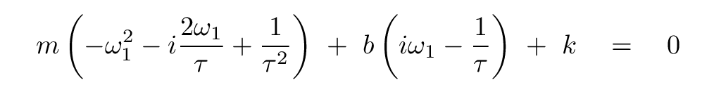
   Use the imaginary parts of this equation to derive a relationship
              for the time constant τ.


   Then use the real parts of this equation to derive a relationship
              for the frequency ω1.
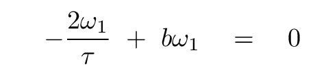
The imaginary parts yield

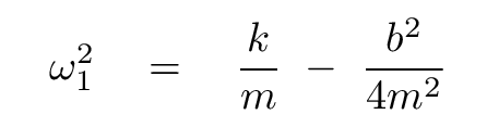
The real parts are

If we substitute our expression for the time constant into these equations, we can derive
Now that we know how to compute the time constant and frequency, we're almost done. Our equation for this combination s1 of the real coordinates x1 and x2 is
But this isn't the only combination of real coordinates that yields a solution to the differential equation. Let's go back to the red box:
Q: What happens if one subtracts the first from the second?

We can now create a new combination by subtracting one block position from the other: s2 = x2 - x1.
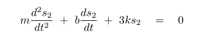
We can follow exactly the same procedure to solve this differential equation for the variable s2. We guess a solution

and plug it into the differential equation. After splitting the result into real and imaginary parts, we can in the same manner derive the time constant and frequency of this motion.

So the time constant is the same in this mode, but the frequency is different.
The definitions of these combinations are

which we can invert to solve for the positions of the two blocks
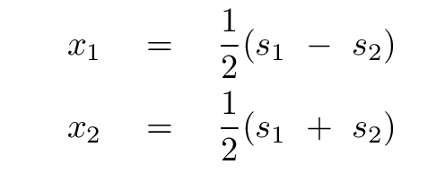
In other words,

Perhaps it will help to understand these equations if we plot the positions of two blocks undergoing damped, coupled harmonic motion. We'll use initial conditions
The first few seconds of motion look similar to that of an undamped system ...
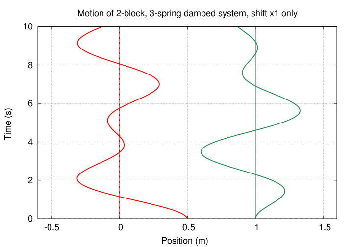
... but after five or ten periods, the amplitude of motion decreases.

But there's another way to reach this same solution to the problem of coupled, damped, oscillators. Let's go back to the force equations in the red box.
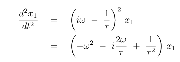
If we guess that the positions will have forms like

then we can express both the first and second derivatives as multiples of the position.
  Q:  What is the first derivative of position with respect to time?

  Q:  What is the second derivative of position with respect to time?

If we use these expressions for the derivatives, then the force equations can be written in matrix form like so:

You should know what to do with this sort of matrix equation by now: look for a solution in the form of a linear combination of the positions,

and thus use the matrix to look for eigenvalues and eigenvectors.
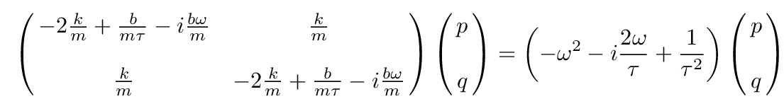
To save some time, instead of going through all the algebra to find the p and q, let's just make a guess, and see if it works.
How about
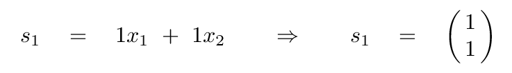
    Q:  Insert p = 1, q = 1 into the matrix equation.  What is
               the resulting time constant and frequency?
After a bit of algebra, you should find familiar results:
Evidently, our guess for the eigenvector was a good one.
Let's push our luck, and guess a second combination of the factors p and q.
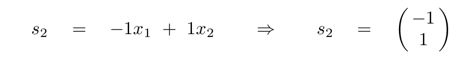
    Q:  Insert p = -1, q = 1 into the matrix equation.  What is
               the resulting time constant and frequency?
Yes, indeed, we end up with the same time constant, and with the frequency
So, in summary, as long as we start by writing correctly the forces on each block, we can take several different mathematical journeys, yet always end up with the same solutions.
Copyright © Michael Richmond.
This work is licensed under a Creative Commons License.