This document describes the steps necessary to set up the Tomoe pipeline, so that one can run it on data taken with the full Tomoe camera. These notes replace the ones in Tomoe Note 010 . That document was written several years ago, and the pipeline has changed in some ways to deal with the new data.
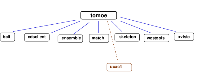
Although it is not strictly necessary, it will make things easier if you create one "top" level directory for Tomoe analysis, and place all the software needed to run the pipeline under this "top." I suggest a structure like this:
These directories are all for the software used to process the data; the "ucac4" directory is a slight exception, as it consists of star catalog files, not code. Because it is larger than the other directories, about 2 GB in size, you might place it in some other location; but it's okay to be underneath the "top" directory as well.
What about directories for the data? There are two types:
The pipeline will NOT MODIFY any of the raw data files in their own directory. So, it is safe to run the code, and run it again, and again, and again; the original raw data is only read, never written or modified.
The pipeline uses software from a number of different packages, so you must copy the code for each package into its directory. All of these are public, open-source packages. You can either copy the versions I've used in June 2019, or try to download more recent versions of some, if you wish. However, it's possible that more recent versions might break some of the pipeline code.
Below is a list of the packages, together with references to the original websites or authors.
Early versions of the Tomoe pipeline used this package to download sections of the UCAC4 stellar catalog, in order to perform astrometric and photometric calibration. The current version still has an option to do so, but using the network is slow; so the new version also has an option to use a local, modified version of the UCAC4 catalog instead. That is much faster and more reliable.
In theory, then, one might not need this package to run the pipeline.
The programs are written in the C language. They rely upon the GNU Scientific Library (GSL), so this package must be installed on the computer as well. See the GSL pages for directions on downloading and installing it. The README file in the ensemble package contains special instructions for building the package if the GSL libraries are not in the regular system directories, but in one of the user's own directories instead.
An example of the format is shown below, for star UCAC4 568-000021.
568-000021 0.17807 23.57824 17.159
Stars are collected in groups by Declination, with one datafile for each 0.2 degrees in Declination.
In addition to the packages listed above, the computer on which one runs the pipeline must have the following software installed:
The "skeleton_2019" directory contains a set of Perl scripts which process Tomoe data, starting with the raw chunk files and producing -- if all goes well -- lists of stars with (RA, Dec) and calibrated V-band magnitudes.
The file run_scripts.pl holds all the basic pipeline functions within it. It is possible to call it directly from the command line, but it will process just one chunk file from a single sensor, such as TMQ1201905290012133543.fits. and then stop. That is not very useful, except for testing purposes.
Most of the time, the goal is to run the pipeline on many chunks, to reduce the data from multiple sensors and over many minutes or hours. For this purpose, the file run_fields_2019.pl is more useful. One can
Let me illustrate this procedure with an example;
cd /gwkiso/tomoesn/richmond/skeleton_2019
@chip_list = ("11", "12");
Next, the list of chunks (file index numbers) to be analyzed
for those sensors.
          my $start_index = 121336;
          my $end_index = 121338;
We need to tell the script where the raw datafiles are located,
and the start of the raw datafile names. Note that the
$raw_file_base contains just the first portions of the
full filename: "TMQ1" means "quadrant 1 of the camera",
and "20190529" is the date.
The full file name then contains the chunk number,
the sensor ID, and the ".fits" extension.
          my $raw_data_dir = "/lustre/tomoesn/realraw/20190529";
          my $raw_file_base = "TMQ120190529";
mkdir /gwkiso/tomoesn/richmond/work/work_20190529
cd /gwkiso/tomoesn/richmond/work/work_20190529
perl /gwkiso/tomoesn/richmond/skeleton_2019/run_fields_2019.pl base=runa debug=1 >& runa.out
We will now look at the output of the pipeline. Although some of the items have changed slightly, Tomoe Note 010: Building the Tomoe pipeline provides a good deal of useful information on the output files. So, you might refer to it if the material below is not sufficient.
After several minutes pass, script finishes. The output directory now contains two items:
runa runa.out
The first, "runa", is a directory which contains all the results of this processing. We'll look at it in a moment. The second, "runa.out", is a simple text file which contains any messages that the pipeline may have printed as it was performing the work. For example, any error messages will be saved on this text file; that is very useful for figuring out what went wrong.
Let's look in the "runa" sub-directory now. It looks like this:
runa_11_00121335  runa_11_12133511.out  runa_12_00121335  runa_12_12133512.out
runa_11_00121336  runa_11_12133611.out  runa_12_00121336  runa_12_12133612.out
runa_11_00121337  runa_11_12133711.out  runa_12_00121337  runa_12_12133712.out
runa_11_00121338  runa_11_12133811.out  runa_12_00121338  runa_12_12133812.out
Once again, there are pairs of items. Each chunk of raw data has
For example, the directory "runa_11_00121335" contains all the results for sensor 11 and chunk 121335; any error messages produced during its analysis can be found in "runa_11_12133511.out".
Here's a picture which may help to illustrate the structure of the output:
       directory for    sub-directory        sub-directory and text file
         one night        one run             for each sensor and chunk
------------------------------------------------------------------------


                                        runa_11_00121335
                                        runa_11_12133511.out
       work_20190529       runa
                                        runa_11_00121336
                                        runa_11_12133611.out

                                        runa_12_00121335
                                        runa_12_12133511.out

                                               etc.
------------------------------------------------------------------------
Let's pick one sensor and chunk -- sensor 11, and chunk 121335 -- and look at the contents of its subdirectory. If we go to the directory "runa_11_00121335" and list the contents, we'll see:
addheader.log              Q_00121335__0003_fits.pht  Q_00121335__0008.fits
pff                        Q_00121335__0004.fits      Q_00121335__0008_fits.coo
Q_00121335__0000.fits      Q_00121335__0004_fits.coo  Q_00121335__0008_fits.pht
Q_00121335__0000_fits.coo  Q_00121335__0004_fits.pht  Q_00121335__0009.fits
Q_00121335__0000_fits.pht  Q_00121335__0005.fits      Q_00121335__0009_fits.coo
Q_00121335__0001.fits      Q_00121335__0005_fits.coo  Q_00121335__0009_fits.pht
Q_00121335__0001_fits.coo  Q_00121335__0005_fits.pht  Q_00121335__0010.fits
Q_00121335__0001_fits.pht  Q_00121335__0006.fits      Q_00121335__0010_fits.coo
Q_00121335__0002.fits      Q_00121335__0006_fits.coo  Q_00121335__0010_fits.pht
Q_00121335__0002_fits.coo  Q_00121335__0006_fits.pht  Q_00121335__0011.fits
Q_00121335__0002_fits.pht  Q_00121335__0007.fits      Q_00121335__0011_fits.coo
Q_00121335__0003.fits      Q_00121335__0007_fits.coo  Q_00121335__0011_fits.pht
Q_00121335__0003_fits.coo  Q_00121335__0007_fits.pht
There are three files for each individual image in this chunk:
There is also one last sub-directory, called "pff". Inside this subdirectory are all the calibrated results. Let's look at it:
multi_match.out            Q_00121335__0004.ast  Q_00121335__0009.ast
multi_Q_00121335__var.out  Q_00121335__0004.pht  Q_00121335__0009.pht
Q_00121335__0000.ast       Q_00121335__0005.ast  Q_00121335__0010.ast
Q_00121335__0000.pht       Q_00121335__0005.pht  Q_00121335__0010.pht
Q_00121335__0001.ast       Q_00121335__0006.ast  Q_00121335__0011.ast
Q_00121335__0001.pht       Q_00121335__0006.pht  Q_00121335__0011.pht
Q_00121335__0002.ast       Q_00121335__0007.ast  solve_Q_00121335__var.cal
Q_00121335__0002.pht       Q_00121335__0007.pht  solve_Q_00121335__var.img
Q_00121335__0003.ast       Q_00121335__0008.ast  solve_Q_00121335__var.out
Q_00121335__0003.pht       Q_00121335__0008.pht  solve_Q_00121335__var.sig
In this directory, there are two files per individual image:
In addition, there are summary files containing a list of stars from ALL the images which were part of the ensemble for this set. The ensemble will only contain objects which appeared in at least 2 images. The interesting ensemble outputs are
Once the pipeline has run successfully, producing lists of many stars with calibrated positions and magnitudes, it is time to sift through the files to find objects which may have suddenly appeared and then disappeared; in other words, to search for transient objects.
The "skeleton" directory contains two scripts which carry out this search. The first is the important one, and the second simply runs the first on a large set of directories.
The first is transient_a.pl, which scans the output files created by the pipeline to look for objects which appear only briefly. One calls it in the following manner.
cd /gwkiso/tomoesn/richmond/work/work_20190529
perl /gwkiso/tomoesn/richmond/skeleton_2019/transient_a.pl prefix=runa_ runa_11_00121335 debug=1 >& transient_a.out
Usually, you will want to search a large number of chunks; perhaps all the chunks generated during a night. You can use wildcard characters in the argument for the chunk to match many chunks at once:
perl /gwkiso/tomoesn/richmond/skeleton_2019/transient_a.pl prefix=runa_ runa_11_???????? debug=1 >& transient_a.out
This procedure may take several minutes or more to finish, if it is analyzing a large number of chunks.
The most important section of this code, inside the file transient_a.pl, is the subroutine called find_transients. Inside this subroutine are lines which set the parameters used to set the properties of "good" transients. For example, this section
  # parameters of the tests that star must pass to qualify as transient
    my $max_mag = $limiting_mag + 1.0;
    my $max_det = 20;
    my $window_extra = 3;
states that in order to qualify as a "good" transient, an object must
Since these and other lines of code within the find_transients routine set the properties of the candidates which will be produced, understanding this routine is very important. If you wish to search for a different type of transient object -- perhaps one which remains bright for a longer time -- then you should edit the code in this routine.
The output of the transient_a.pl script is a text file with one line per candidate object. Each line looks something like this:
# trans 1 chunk 0109500 star 226 798 2089 = 196.18406 -16.13120 16.184 0.74 6 349 354
The columns are
The second script can help you to look through a long list of candidate transient objects quickly. It takes a list of candidate transient objects as input, and generates an HTML document with both a listing of all the information shown above, plus small image cutouts of each detection of every candidate. This is the show_trans.pl script.
The basic usage is
perl /gwkiso/tomoesn/richmond/skeleton_2019/show_trans.pl transient_a.out html=1 debug=1 >& show_trans.out
You can find an example of the documents created by this routine in Tech Note 9:
Examining this document by eye will often reveal that some candidates are not real transient objects, but simply faint stars which are usually just below the detection limit, or perhaps moving objects. See the discussion in Tech Note 9 for more details.