Tomoe Note 010: Building the Tomoe pipeline
Michael Richmond
Jun 19, 2017
This document describes how one can acquire all the software
necessary to run a pipeline on a set of Tomoe data,
set it up properly on one's computer,
and then run the pipeline.
One must grab the following software packages onto
one's computer:
-
cdsclient
- This package allows one to grab data from the catalogs
at the
Strasbourg astronomical Data Center .
In particular, we need to select stars with good
positions and magnitudes to calibrate the
Tomoe images.
I have used version 3.8.3 for my tests,
so later versions will probably work, too.
-
ensemble
- This package (which I wrote) analyzes the photometry
from many images of the same field,
performing inhomogeneous ensemble photometry
as described in
Honeycutt, PASP 104, 435 (1992).
In order to perform some linear algebra,
this package calls routines which are part of
the GNU Scientific Library ,
so it is necessary to install that package
on one's computer first (if it has not already
been installed).
After downloading and unpacking the "ensemble" code,
you must build it. Go to the directory
containing the code and type
                ./configure
                make
                make check
If all goes well, there will be no errors in the
compiling, and the final comment should yield a result
that looks something like this:
            make  check-TESTS
            make[1]: Entering directory `/w/tomoe/temp/ensemble-1.0'
            selftest.pl: passes all test okay
            PASS: selftest.pl
            ==================
            All 1 tests passed
            ==================
-
match
- This package (which I wrote) compares one set of stars
to a second set, and looks for a transformation
(translation, rotation, scaling)
which brings the two sets into alignment.
After downloading and unpacking the code,
you must build it. Go to the directory
containing the code and type
                ./configure
                make
                make check
If all goes well, there will be no errors in the
compiling, and the final comment should yield a result
that looks something like this:
            make  check-TESTS
            make[1]: Entering directory `/w/tomoe/temp/match-1.0'
            match: passed all tests
            PASS: selftest.pl
            =============
            1 test passed
            =============
-
WCSTools
- This package performs many operations on FITS
files, especially dealing with FITS header information
and coordinate transformations.
I have used version 3.9.4 for my tests,
so later versions will probably work, too.
After downloading and unpacking the code,
you must build it. Go to the directory
containing the code and type
make all
If all goes well, there will be no errors in the
compiling.
-
xvista
- This package (which I wrote) contains a number of
programs for manipulating and analyzing
FITS images.
It performs the image arithmetic needed to clean
the raw images,
and finds and measures the properties of stars in
the clean images.
After downloading and unpacking the code,
you must build it. Go to the directory
containing the code and type
                ./configure
                make
                make check
If all goes well, there will be no errors in the
compiling, and the final comment should yield a result
that looks something like this:
               make  check-TESTS
               make[2]: Entering directory `/w/tomoe/temp/xvista-0.1.13'
               PASS: selftest.pl
               =============
               1 test passed
               =============
-
skeleton
- This package (which I wrote) contains Perl scripts
which contain the "glue" to combine programs
from all the other packages in the proper way
to run the entire pipeline.
-
gnuplot
-
ImageMagick
It might be convenient to place all the packages
into a single directory. If you do so,
after you have unpacked and built them all,
that directory might look something like this:
$ /bin/ls
cdsclient-3.84  match-1.0     wcstools-3.9.5
ensemble-1.0    skeleton-0.1  xvista-0.1.13
Note that on my system, the
"gnuplot" and "ImageMagick" packages had already been
installed in another directory
(/usr/bin),
so they do not appear here.
The pipeline needs to know where these external software
programs are on the computer,
so it is necessary to edit one of the "skeleton"
scripts and insert this information.
Go to the "skeleton" directory and edit the file tomoe_config.pl.
You should see a section like this:
#    XVista: image processing programs
xvista_dir     => "/w/tomoe/xvista",
#    match: matching star lists
match_dir      => "/w/tomoe/match",
#    ensemble: inhomogeneous ensemble photometry
ensemble_dir   => "/w/tomoe/ensemble",
#    WCS: World Coordinate System tools
wcs_dir        => "/w/tomoe/wcstools/wcstools-3.9.4/bin",
#    CDS: tools to grab star catalog data from CDS websites
cdsclient_dir  => "/w/tomoe/cdsclient/cdsclient-3.83",
#    scripts: home of the scripts in the Tomoe pipeline
script_dir     => "/w/tomoe/skeleton-0.1",
#    gnuplot: home of the gnuplot executable program
gnuplot_dir     => "/usr/bin",
#    convert: home of the ImageMagick 'convert' executable program
convert_dir     => "/usr/bin",
Edit this section so that each line contains
the full path to the location of the packages
on your system.
For example, when I was testing the pipeline,
my file looked like this:
#    XVista: image processing programs
xvista_dir     => "/w/tomoe/temp/xvista-0.1.13",
#    match: matching star lists
match_dir      => "/w/tomoe/temp/match-1.0",
#    ensemble: inhomogeneous ensemble photometry
ensemble_dir   => "/w/tomoe/temp/ensemble-1.0",
#    WCS: World Coordinate System tools
wcs_dir        => "/w/tomoe/temp/wcstools-3.9.5/bin",
#    CDS: tools to grab star catalog data from CDS websites
cdsclient_dir  => "/w/tomoe/temp/cdsclient-3.84",
#    scripts: home of the scripts in the Tomoe pipeline
script_dir     => "/w/tomoe/temp/skeleton-0.1",
#    gnuplot: home of the gnuplot executable program
gnuplot_dir     => "/usr/bin",
#    convert: home of the ImageMagick 'convert' executable program
convert_dir     => "/usr/bin",
The tomoe_config.pl file has some additional
parameters which describe general properties of the
images; for example,
the location and number of overscan rows,
or the plate scale in arcseconds per pixel.
If the properties of the camera have changed since
this software was written,
it may be necessary to modify some of these parameters.
The Tomoe camera produces large FITS files
which contain a number of individual FITS images.
I will use the term "composite" to describe these
large, raw datafiles.
The word chunk
refers to all the measurements recorded in
this composite file.
In this example, I'll use a single
composite file as the input.
On my computer,
it sits in the directory /w/tomoe/temp/data:
$ /bin/ls -l /w/tomoe/temp/data
-rwxr-xr-x 1 richmond richmond 1866248640 Dec  1  2016 TMPM0109330.fits
The composite file is named TMPM0109330.fits.
This standard name has a particular format:
                TMPM      010933       0     .fits
                 ^           ^         ^       ^
                 |           |         |       |
                 |           |         |       suffix
                 |           |         |
                 |           |        chip index (0-7)
                 |           |
                 |          frame index (always increasing)
                 |
                 prefix
A typical composite file contains 360 images from a single chip.
For images with an exposure time of 0.5 seconds,
the entire file covers a span of 180 seconds = 3 minutes.
So, during a night of length 8 hours = 480 minutes,
each chip would produce (480 / 3) = 160 frames,
and 160 composite files;
that means that the "frame index" number would increase by 160
during the course of the night.
Each chip produces separate composite files.
The prototype camera used during 2016 had 8 chips,
so the chip values range from 0 to 7.
When larger versions of the camera are built,
the name convention will have to change;
perhaps two characters will be used to denote the chip number.
In order to run the pipeline,
one should create a directory into which all
temporary and permanent pipeline output will be placed.
For this example,
I'll create a directory called work for this purpose.
$ cd /w/tomoe/temp
$ mkdir work
$ /bin/ls
cdsclient-3.84  ensemble-1.0  skeleton-0.1    work
data            match-1.0     wcstools-3.9.5  xvista-0.1.13
Before running the pipeline,
we can choose to "de-activate"
some sub-sections of it.
The entire pipeline has a number of "stages",
which are carried out in sequence on every image.
There may be times when you wish to perform
only one or two of the stages;
for example,
if you have already run the stage which extracts
individual FITS images from the composite files,
and saved the FITS images,
you can skip that stage.
To "activate" or "de-activate" particular stages,
edit the run_scripts.pl file.
Around line 148,
there is a section which looks like this:
# which pieces of the pipeline do we want to activate?
#
# split composite FITS files into individual images?
$do_split = 1;
# subtract the bias from raw images?
$do_sub_bias = 1;
# find and measure stars in each clean image?
$do_stars = 1;
# add JD to the starlist files?
$do_addjd = 1;
# run the ensemble photometry programs?
$do_ensemble = 1;
# calibrate the ensemble output?
$do_calib_ensemble = 1;
# calibrate the individual .pht files?
$do_calib_pht = 1;
# create diagnostic graphs?
$do_make_graphs = 1;
The value "1" indicates that a stage is "active" and will run.
By default,
the pipeline will run every stage.
In order to "de-activate" a stage,
set the value of its line to 0.
For example, to skip the stage which splits composite FITS files
into individual images,
I would edit the file so it looked like this:
# split composite FITS files into individual images?
$do_split = 0;
There are several ways to run the pipeline,
but a simple one is as follows:
- cd to a directory into which all the
pipeline output will go
cd work
- invoke the run_scripts.pl script
in something like the following manner:
    perl ../skeleton-0.1/run_scripts.pl  ../data/TMPM0109330.fits
              basedir=test_  config_dir=../skeleton-0.1  debug=1   >&  run_scripts.out
Let's look at the pieces of that rather long command.
- First, the command perl, because
the scripts are written in the Perl language.
If you choose to make the scripts executable,
you don't need to start with this
- Next, the full name of the run_scripts.pl
script, including a relative or absolute path
to it
- The next argument(s) is the name(s) of a raw composite
FITS file. To reduce multiple files,
just add their names here
- The next argument provides the prefix of a sub-directory
into which all the pipeline output will be placed;
the end of the directory's name is the frame
index plus chip number.
In this example, the command is being executed
in the work directory, and all output
will be placed into a sub-directory called
test_0109330.
If we supplied multiple composite data files
as input arguments, then multiple sub-directories
would be created, each one starting with the
string test_; for example,
test_0109330, test_0109340, and so forth.
- The next argument is the name of a directory
which contains the tomoe_config.pl
file, which in turn contains a number of
parameter=value pairs (such as the names
of the directories with external packages)
- The final argument in this example sets the
debug level of the output. By default, the
pipeline prints very little as it executes,
aside from any warning or error messages;
this is equivalent to debug=0.
By setting debug=1,
the pipeline will print many, many diagnostic
messages describing its progress as it executes.
The current version, for example, produces
roughly 60,000 lines and 4.6 MBytes of output.
Using debug=2 will produce even more output.
- The final words in the command above re-direct the
(very verbose) diagnostic messages into a
file called run_scripts.out.
On my current machine, which runs on an Intel i7-4790 CPU @ 3.60GHz
rated at 7183 bogomips,
a single composite FITS file takes about 2.5 minutes to process
completely.
If you run the pipeline with a debug level of 1 or higher,
then all the temporary files produced will still be present;
there can be many hundreds of them for each composite FITS file.
In general, these temporary files have names of the form
do_something_XXXXX,
where the XXXXX are five random alphanumeric characters.
A quick way to delete all temporary files
is to run the del_tempfiles.pl script:
perl ../skeleton-0.1/del_tempfiles.pl
If the pipeline is run with debug=0,
then it will automatically delete all temporary files
after they are no longer needed.
For each input composite FITS file,
the pipeline will create a separate directory
for all output files.
In my example, the output file for frame 010933, chip 0,
has name test_0109330.
Inside this directory,
there should five files per individual FITS image,
plus one sub-directory
with calibrated quantities.
- For each individual FITS image, there will be
five output files with very similar names.
In my example, the composite FITS file
contains 360 individual images, which are
numbered 0 - 359. The image number 100
gives rise to the following output files:
- Q_0109330__0100.fits is a cleaned version
of the FITS image
- Q_0109330__0100_slice.fits is a small
FITS image which contains a single
unit of the bias signal for the frame.
This small unit is repeated to create
a full-size image, which is subtracted from
the raw image to produce the "clean" image.
- Q_0109330__0100_slice.fits.msk is a
"mask" version of the bias image:
pixels are either 0 (signalling "good")
or 1 (signalling "bad").
This information is not used by the current
version of the pipeline, but may be in the future.
- Q_0109330__0100_fits.coo
is a list of objects found in the image,
Each object has a position (in pixels),
a local background value (in counts per pixel),
peak pixel value above sky (in counts),
FWHM (in pixels),
roundness, and sharpness.
See the stars command of the
XVista package
for more information on these values.
This file is not used in any further pipeline
processing, but it can be very useful to
diagnose problems with the pipeline,
or to determine the best values of several parameters
for finding stars.
- Q_0109330__0100_fits.pht
is a list of the same objects, but this
time with raw photometry for each object;
that is, an uncalibrated measure of its brightness
through one or more synthetic apertures.
The size of these apertures can be set using the
var_aper_factor and fixed_aper_rad
values in stars.pl.
See the phot command of the
XVista package
for more information on the
format of each line of this file.
This file IS the basis for all further
pipeline stages and output.
- The single sub-directory has the name pff.
Inside are slightly modified copies of the .pht
files for each individual image,
as well as a small number of additional
files.
- Q_0109330__0100_fits.pht
is an example of the .pht file corresponding
to each FITS image.
This version has one additional column,
which contains the Julian Date of the measurement.
- Q_0109330__0100_fits.ast
is an example of the .ast file corresponding
to each FITS image.
This is similar to the .pht file, but
contains calibrated quantities:
position in (RA, Dec) instead of pixels,
and calibrated (V-band) magnitude instead
instrumental magnitude
- multi_match.out
contains information pertaining to the
multipht program, which tries to
find a simple translation to bring each
image into registration with the others.
- multi_Q_0109330__var.out
is a file which is created by the multipht
program, and used as input by the
solvepht program.
- solve_Q_0109330__var.out
is a single file containing calibrated
output from the solvepht
ensemble photometry program:
positions in (RA, Dec) and calibrated V-band magnitude.
Only stars which are members of the ensemble
(meaning stars which appear in at least N images within
this chunk of data)
will appear in this file.
The value of N is set by the
star_cut parameter, defined in do_multi.pl.
- three files containing output from the solvepht
ensemble photometry program, with names like
- solve_Q_0109330__var.out
- solve_Q_0109330__var.img
- solve_Q_0109330__var.sig
See documentation for the
ensemble package
for more information on these files.
- five graphs are produced by the final stage of the
pipeline, providing quick diagnostic information.
Each graph appears in two forms, as Postscript
and PNG:
- numobj_0109330_var.ps, numobj_0109330_var.png
- emplot_Q_0109330__var.ps, emplot_Q_0109330__var.png
- emplot_cal_0109330_var.ps, emplot_cal_0109330_var.png
- magsig_Q_0109330__var.ps, magsig_Q_0109330__var.png
- magsig_cal_Q_0109330__var.ps, magsig_cal_Q_0109330__var.png
Examples of these five graphs are shown below.
Note the slight redundancy in this output.
Identical measurements of most stars will appear in two places.
First, in the .ast file
corresponding to each image;
every star, even if it is detected only in a single image,
will have calibrated measurements in an .ast file.
Stars which are detected enough times to become members
of the photometric ensemble will ALSO appear in the
single
solve_Q_xxxxxxx__var.out
for this chunk.
Since all the measurements for a given star are collected
together in the
solve_Q_xxxxxxx__var.out
file,
that is usually a more convenient
place to start detailed analysis than
the individual .ast files for each image.
A quick way to find out if a run of the pipeline has succeeded
is to examine these output files.
Check to see if the pff directory exists
and contains 5 .png files.
If not, some of the processing probably failed.
If these .png files do exist, then examine each one
briefly and see if it has the proper general form.
Below are examples of graphs from a successful run.
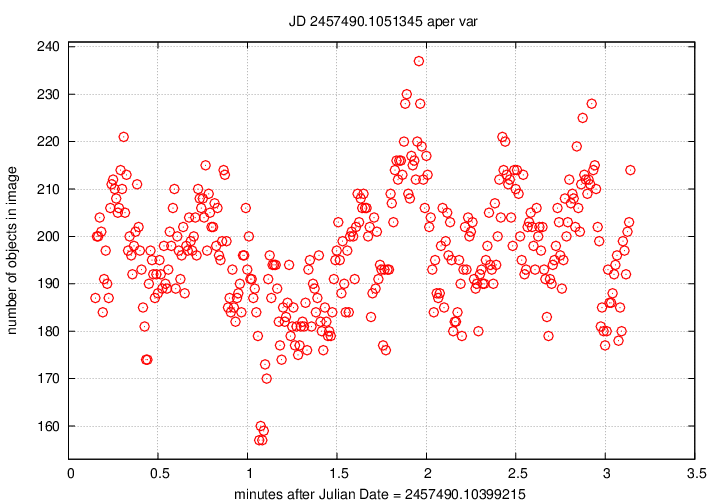
The numobj_xxxxxxx_var.png plot is
the simplest:
it shows the number of objects detected in each
individual FITS image of the chunk,
as a function of time from the start of the chunk.
For typical prototype datasets,
each chunk lasts about 3 minutes,
and good conditions should produce 100 - 300
objects per image.
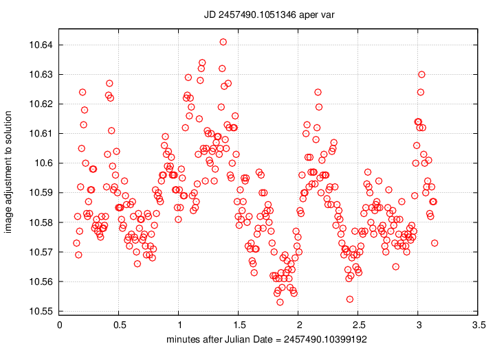
Two graphs primarily indicate the presence (or absence) of
clouds during the observations.
The emplot_Q_xxxxxxx__var.png graph
displays on the vertical axis a measure of the difference
between the instrumental magnitudes of stars in each
image, and the AVERAGE instrumental magnitudes of those
stars in the ensemble of all images in the chunk.
For example, if a cloud appears near the end of a chunk's
exposures, the stars in those images will be dimmer
than average; dimmer stars mean larger magnitudes, so the
difference
image adjustment = (mag in this image) - (average mag)
will be positive.
In the example below, note the dip in this graph just before
2 minutes after the start --
that indicates that all the stars appeared a bit brighter
than average: the telescope was looking through a break
in thin clouds. In the numobj graph above, note that
more stars were detected at that time.
But after the 2-minute mark, the emplot graph
rises, indicating that stars become dimmer due to clouds;
the number of stars detected drops at this same time.
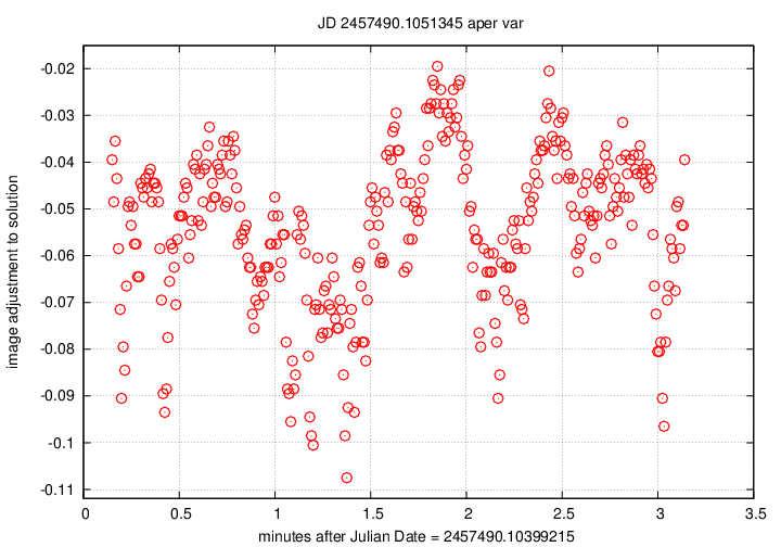
The emplot_cal_xxxxxxx_var.png
is very similar: it also shows the difference between
the magnitudes of stars in each individual image,
and the average over the course of the chunk.
However, the zeropoint of these values is different:
it is tied to the calibrated magnitudes of the stars
in a photometric reference catalog, rather than simply
the average instrumental value in the ensemble.
There is a second difference: the SIGN of the
difference has been switched, so that the vertical
axis shows a quantity with the sense
image adjustment = (calibrated mag) - (mag in this image)
This is certainly confusing.
Future versions of the pipeline should adopt a single
convention for both graphs.
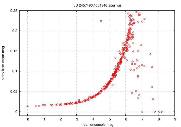
The final pair of graphs again show a similar quantity,
with just a small difference.
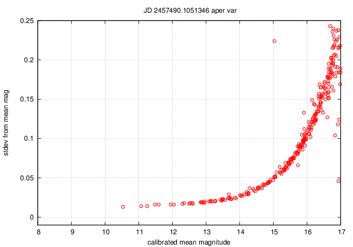
magsig_Q_xxxxxxx__var.png
shows the scatter in measurements of each star
in the photometric ensemble as a function of its brightness.
Bright stars (on the left) should have small scatter,
and faint stars (on the right) should have large scatter.
Positive outliers, such as the single high point
close to mag = 4.5 in the example below,
may be variable objects.
The magsig_cal_xxxxxxx_var.png
graph is almost identical.
The only difference is the zeropoint of the horizontal axis.
In the previous graph, the brightest star in the ensemble
is assigned a magnitude value of zero;
but in the magsig_cal version,
the stars are calibrated properly against photometric reference
catalogs.
The range for typical Tomoe data should be from about magnitude 8
to about magnitude 17.
The method
described above
will process a single composite file,
or several such files.
But it can be awkward to use on an entire night of data.
Therefore, there is another script,
run_fields.pl,
which is designed to call the basic
run_scripts.pl
repeatedly on a large number of composite FITS files.
My usual procedure is to consider the data from
each chip of the detector as an independent set.
So, for example,
let's consider all the images taken
with chip 0 on the night of 20160411 = April 11, 2016.
On my system, these files can be found in the directory
/media/root/tomoepm201604/20160411.
There are 126 composite FITS files:
  TMPM0108830.fits
  TMPM0108840.fits
  TMPM0108850.fits
    ...
  TMPM0110060.fits
  TMPM0110070.fits
  TMPM0110080.fits
Note that the first file has index number 10883,
and the last has index number 11008.
In order to run the pipeline on all these files,
we can invoke the run_fields.pl script as follows:
   perl ../skeleton-0.1/run_fields.pl chip=0 base=testa_
       start=10883 end=11008 raw_file_base=TMPM0
       datadir=/media/root/tomoepm201604/20160411
       config_dir=../skeleton-0.1 debug=1  >&  run_fields_testa.out
The arguments to this command are
After processing an entire night's worth of data, just for one chip,
one may have over 100 directories, each with hundreds of data files.
Is there any easy way to find out if the results are good,
or if they suffered from bad weather or equipment failure?
Yes.
The check_weather.pl script looks at output of the
pipeline, computes a number of summary statistics,
and creates a single graph which shows several quantities
as a function of time during the night.
One can learn much about the conditions of the sky
and the data with a quick glance at this graph.
One can find detailed descriptions of this script and its
graphical output at
To run the script, go to the directory
in which the sub-directories for each chunk are located.
In my example, this is the work directory.
     $ pwd
     /w/tomoe/temp/work
     $ /bin/ls -d testa_*
     testa_0109300  testa_0109360     testa_109310.out  testa_109370.out
     testa_0109310  testa_0109370     testa_109320.out  testa_109380.out
     testa_0109320  testa_0109380     testa_109330.out  testa_109390.out
     testa_0109330  testa_0109390     testa_109340.out  testa_109400.out
     testa_0109340  testa_0109400     testa_109350.out
     testa_0109350  testa_109300.out  testa_109360.out
I ran the pipeline on a dataset containing 11 chunks, numbers 010930 to 010940,
all with chip 0 only.
There are therefore 11 subdirectories, one for each chunk,
with the prefix testa_.
There are also 11 pipeline output files, one for each chunk,
with the same prefix; the output files have suffix .out.
In order to check the output from these 11 chunks,
I can run the check_weather.pl script like so:
     $ perl ../skeleton-0.1/check_weather.pl prefix=testa_
             testa_01093?0 testa_0109400
             config_dir=../skeleton-0.1
             debug=1 >& check_weather.out
The arguments here are:
After running the script, three new files are created.
One is the check_weather.out file with
diagnostic information,
and the other two contain the graphs produced by this routine.
In this case, they are
- check_weather_0109300_0109400.png
- check_weather_0109300_0109400.ps
Note that the names include the (chunk index) + (chip) numbers
for the first and last sub-directory included in the analysis.
To illustrate features of the graphs produced by this routine,
I'll choose one from
Tech Note 007
which contains results for an entire night.
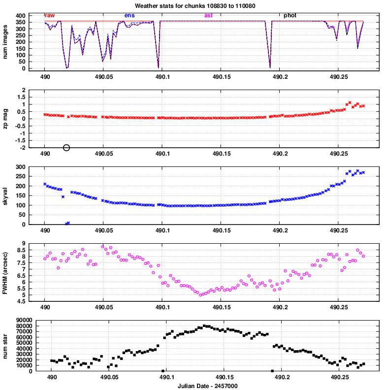
The five panels, from top to bottom,
illustrate various features in the reduced data.
- number of images: the number of chunks which passed successfully
through various stages of the pipeline.
The four line colors show how many chunks were in the
raw input set, were processed through the ensemble analysis,
were successfully matched to astrometric catalogs,
were successfully matched to photometric catalogs.
- zeropoint: the difference between the instrumental magnitudes
and calibrated magnitudes for stars in each chunk.
Large positive numbers indicate less light reaching
the detector.
- skyval: counts per pixel in the background sky.
- FWHM: typical Full-Width-at-Half-Maximum, in arcseconds
- number of stars: number of objects detected in a chunk,
adding together objects in all the individual images
in that chunk.
In this particular instance,
it is clear that conditions were best in the middle
of the night.