The term "flatfielding" means something like this:
correcting instrumental photometry for the several types of error as a function of position on the detector
There are a number of sources of error; not all of them act in the same manner, and so not all can be removed by the same sort of correction. The major ones are
The standard practice in astronomy is to take pictures of a bright source of uniform illumination, and assume that any variations in brightness across the resulting image are due to multiplicative errors. One divides a raw image by a normalized version of this "flatfield image" to remove the errors. If any non-multiplicative errors occur in the optical system, such as scattered light, then this "correction" will produce errors in the final photometry.
"Starflats" check the validity of ordinary flatfielding corrections by using stars as sources of constant light. One takes a series of images at slightly different pointings, so that (many) stars appear at many different locations on the detector(s). One assumes that (most of) the stars remain constant in luminosity throughout the procedure, which means that they ought to have identical magnitudes in this set of corrected, dithered images. If there are repeated errors systematically as a function of position on the focal plane, one may conclude that the flatfielding has not been adequate.
An early paper describing this technique is by Manfroid, Stellar calibration of CCD flat fielding , A&A Suppl, 113, 587 (1995).
As described in this earlier technical note, the basic idea is to model the spatial errors in photometry as a relatively simple function of position on the focal plane -- say, as a polynomial of second-order in (x, y) -- set then solve for the values of the coefficients which provide the best fit to the observations. One can then apply the corrections from this model to one's photometry from the ostensibly "corrected" images.
A more recent paper showing this technique in action describes The ELIXIR system at the CFHT on Mauna Kea. The authors show how a mosaic camera with a large field of view suffers from scattered light, and how they can remove its effects.
In order to investigate the signatures of various sources of error on the SNAP photometry, I have been building a simplified photometric pipeline. It does not go down the pixel level, quite, but will allow us to insert various types of error and see how they affect the measured instrumental magnitudes. You can read more about the pipeline in earlier technical notes:
The pipeline is written mostly in the language TCL, but incoporates a few programs written in C. It uses the Tk library for graphical output, but most of it does not include any graphics and can be run without it. Following the example of the SDSS, the pipeline is split into two portions: code and parameters. The parameters are stored in simple ASCII text files, like this:
#
# parameters associated with the filters on the SNAP camera.
#

# input directory, holding fiducial filter tranmission curves
input_dir    /xz/snap/input

# output directory, which will hold transmission curves for
#   actual filters on the spacecraft
output_dir    /xz/snap/output

# number of fiducial filters
num_fiducial 9

# base of the fiducial filter name; the file name has a name
#   like this:  baseN.filter
fiducial_base         fiducial_b
One can easily and quickly modify the parameters without delving into the code; it should be relatively easy for someone to read over documentation, then modify and run the pipeline without having to understand TCL or edit any of the source code.
As of early July, 2004, the pipeline includes
One can create a list of stars in the sky, either by reading from real data in a catalog, or by generating an artificial set of stars with desired properties, and then "observe" them once or many times. The output includes both the instrumental magnitudes and the "expected" magnitudes, which are based on a convolution of the input spectra with the fiducial filter bandpasses. One can then examine the differences between expected and observed magnitude for systematic variations.
In real life, the focal plane would look something like this:
For testing purposes, however, one can create simpler versions, in which all detectors are the same type and all filters are identical (fiducial filter number 5, the reddest one over CCDs):
For an example, I made a catalog of identical stars fallling in a very convenient pattern, sampling each detector in a 4x4 pattern:
I ran light from these stars though the pipeline, recording both the "expected" magnitude for each star (based on the fiducial filter bandpasses) and the measured magnitude. In this run, the only effect I included was the shift in effective bandpass as a function of angle of incidence on the filter. The output provides a clear picture of the signature of shifting filters:
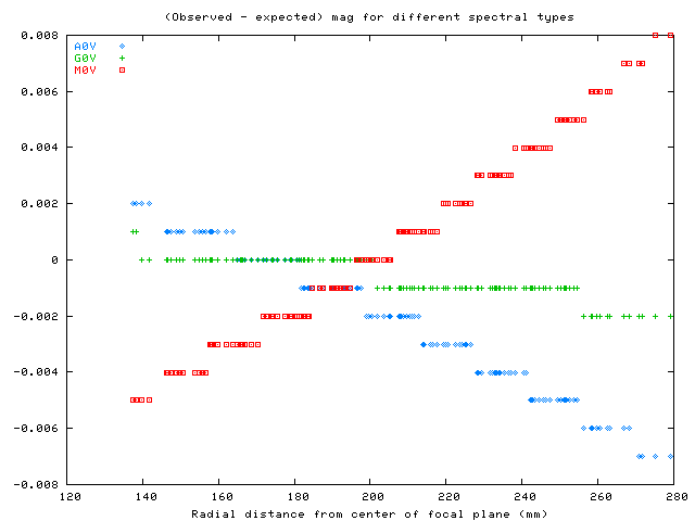
The differences appear in step-like patterns in this graph because I recorded the magnitudes to only three places after the decimal point. Note that hot stars appear fainter near the center, while cool stars appear brighter near the center. This is the same pattern Steve Kent and I determined in earlier work.
Generating simulated measurements of stars is the hardest part, but it isn't the end of the analysis. Once one has a set of output magnitudes, one must run them through a giant least-squares routine to solve for the best-fit values of the model parameters. As shown in a tech note from Oct 22, 2003, one might have an equation as complicated as this:
          M   =   m   +  a    +  b1  * (color)  +  b2  * theta * (color)
                          i        j                 j


                                                 2
                      +  p1  * row   +  p2  * row    +
                           i              i

                                                 2
                      +  p3  * col   +  p4  * col    +
                           i              i

                                               2
                      +  q1  * x     +  q2  * x      +


                                               2
                      +  q3  * y     +  q4  * y
However, at the moment, I have written software to solve for the much simpler equation
          M   =   m   +  a    +   d
                   ij     i        j
where
           M          is the true magnitude of each star

           m          is the observed magnitude in image i on chip j
            ij

           a          is the zeropoint of image i
            i

           d          is the offset of chip j
            j
I have verified that the code finds the proper solution for this case. In the future, I will gradually build up to include more and more complicated photometric equations.