 Copyright © Michael Richmond.
This work is licensed under a Creative Commons License.
Copyright © Michael Richmond.
This work is licensed under a Creative Commons License.
In 1966, Time magazine placed an astronomer on its cover:
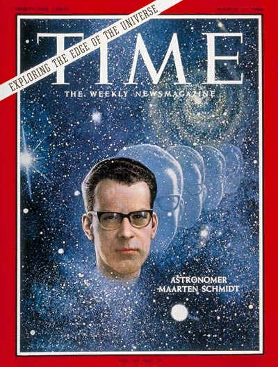
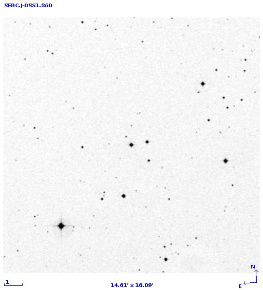
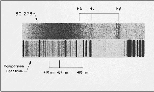
What was his claim to fame? The decoding of the spectrum of quasars -- well, of one quasar, 3C273, anyway. These mysterious radio sources had been discovered only a few years earlier, and a set of fortuitous lunar occultations of 3C273 allowed astronomers to narrow down the location of the radio source to this insignificant little star:
Schmidt used the 200-inch telescope on Mount Palomar to take spectra of this object. He found an indistinct set of emission lines -- the picture below is shown in inverted colors, so that "black" on the picture really means a region with lots of light. I've marked three wavelengths on the picture, in Angstroms, to give you some notion of the scale -- you can assume that there's a constant dispersion across the spectrum, so interpolate between the marked wavelengths.
   Q:  What are the wavelengths of the 3 strongest
       emission lines?


       Can you name the rest wavelengths of these lines?
       (Hint: think hydrogen)


       What is the redshift of this object?
One of the big differences between AGN and quasars, on the one hand, and regular old galaxies, on the other, is luminosity: AGN emit much more energy, at all wavelengths. An obvious consequence is that AGN such as quasars will in general be visible at much larger distances than ordinary galaxies. If one is trying to map out the structure of the universe on large scales, that extra range can make a big difference.
Consider this luminosity function for ordinary galaxies, based on measurements in the SDSS.
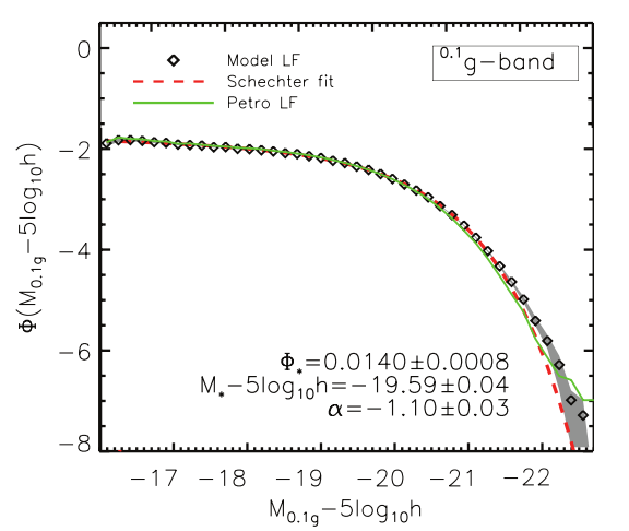
Figure taken and reversed left-right from
Montaro-Dorta and Prado, MNRAS 399, 1106 (2009)
   Q: What are the parameters for the Schechter
      luminosity function fitted to this dataset?

      Click on the figure above to see the values
      from its paper.
Compare that luminosity function to this one, which is again based on SDSS data, but this time measurements of quasars, not ordinary galaxies.
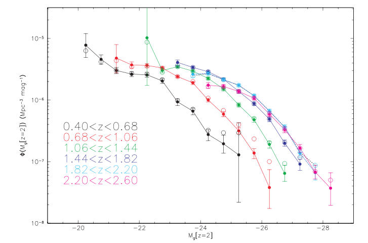
Figure taken from
Croom et al., MNRAS 399, 1755 (2009)
   Q: What are the parameters for the Schechter
      luminosity function fitted to this dataset?
      Use the green points, corresponding to
      objects at 1.06 < z < 1.44.


   Q: How much more distant will a "typical" quasar
      be than a "typical" galaxy in a magnitude-limited
      survey?
Cosmologists often use galaxies as tracers of structure in the universe. One of the tools they employ is the "two-point correlation function", which measures the likelihood that if we look at some particular distance away from a galaxy, we will find another galaxy; more precisely, it expresses the extra likelihood, above that of random chance, that we will find another galaxy at that particular distance from the first.
To measure this correlation function, astronomers must first identify a sample of objects. If the sample spans a region 50 Mpc across, then the largest possible distance over which correlation can be measured is ... 50 Mpc. Clearly, the larger the volume of space over which the objects are spread, the larger the scale over which we can measure this mathematical quantity.
Here's an example of the two-point correlation function for galaxies, based on samples from the SDSS.
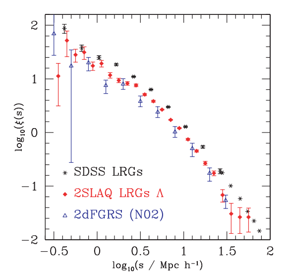
Figure taken from
Ross et al., MNRAS 381, 573 (2007)
Now let's look at the two-point correlation function of quasars, again from the SDSS. The figure below isn't a very good comparison, since the quantity being plotted on the vertical axis isn't the same as the one above, but look at the horizontal axis.
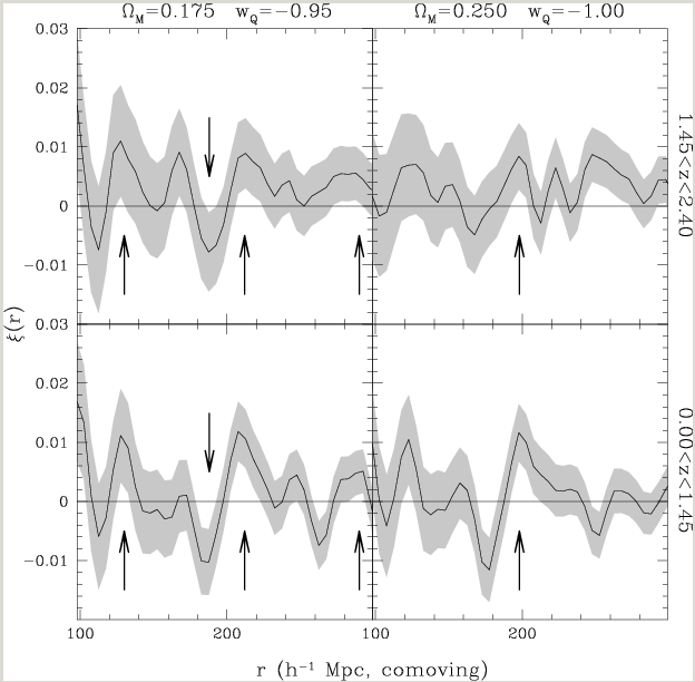
Figure taken from
Zandivarez and Martínez, A&A 498, 347 (2009)
There are many objects in the distant universe which we would love to investigate ... but which are just too faint for us to detect. The radiation they emit may be lost in the general background noise due to light from the Earth's atmosphere, zodiacal light, the interstellar medium, and so forth; or it simply may add up to so few photons per second that we would need to integrate for days just to detect a set of 10 photons.
Quasars to the rescue! Quasars and other AGN produce huge amounts of energy, providing all the photons we need to beat small-number statistics. When a quasar lies behind some interesting object in space, then the light from that quasar must pass through the interesting object. If the material in the object absorbs some of the quasar's light, then we will see absorption lines in the quasar's spectrum.
Image courtesy of
Wallace Sargent at CalTech.
For example, consider the case of the quasar 0229+131. Just a small angle away from it on the sky lies a spiral galaxy.

Image taken from
Kacprzak et al., ApJ 711, 533 (2010)
We can see two faint spiral arms around the galaxy, but neither one extends as far as the QSO .... or so it seems. A spectrum of light emitted by the galaxy shows a shift in the wavelength as a function of position: the galaxy is rotating! In the graph below, the shift in wavelength has been translated into a velocity relative to the center of the galaxy, with units of km/sec.

Image taken from
Kacprzak et al., ApJ 711, 533 (2010)
Q: What is the velocity of the material closest to the QSO?
Now, if we take a spectrum of the quasar, we'll see lots and lots of absorption lines from all sorts of material between it and us. But if we look at wavelengths appropriate for MgII atoms absorbing light at a redshift of z=0.4167, we see .... strong absorption lines at a velocity of about +150 km/sec relative to the center of the galaxy. In other words, we can detect the presence of material in the galaxy which is otherwise invisible. Better yet, if we can detect and resolve several absorption lines, we can determine some properties of the gas.
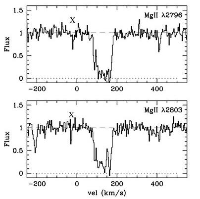
Image taken from
Kacprzak et al., ApJ 711, 533 (2010)
If we look at the spectra of quasars, starting at low redshift and moving to high redshift, we see a systematic change. The Earth's atmosphere transmits only a small range of wavelengths, from about 4000 Angstroms to about 8000 Angstroms, but that range samples a different portion of the rest-frame spectrum of low-redshift and high-redshift quasars.
As we look at quasars at higher and higher redshifts, we see light which was originally emitted at shorter and shorter wavelengths -- in the UV portion of the spectrum. The Lyman-alpha emission line of hydrogen is often the strongest feature, at 1216 Angstroms in the rest frame. If you look to even shorter rest wavelengths, you may notice two aspects of quasar spectra.
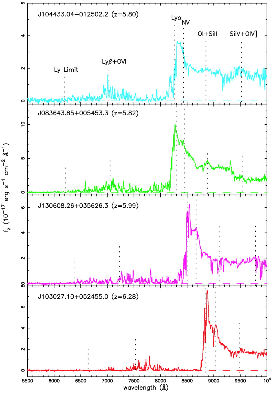
Figure taken from
Becker et al., AJ 122, 285 (2001)
   Q:  Use the energy levels of the hydrogen atom
       to explain the process by which a Lyman-alpha
       photon is emitted, or absorbed.


   Q:  Why is there little light at wavelengths
       shorter than the Lyman-alpha line?


   Q:  Why is there NO light at wavelengths
       shorter than the Lyman limit?
The reason that so little far-UV radiation reaches us is that neutral hydrogen is a very good absorber of any photons with an energy greater than that of Lyman-alpha. Most of the atoms in a cool intergalactic cloud will be in the ground state, which allows them to absorb light with a wavelength of 1216 Angstroms. Clouds at different redshifts -- between us and the quasar -- will absorb light of different wavelengths.
   if QSO redshift      and cloud redshift     we see absorption
   is z=                 is z=                   at wavelength
--------------------------------------------------------------------
     5.0                    4.9

     5.0                    4.7

     5.0                    4.3

     5.0                    3.5

     5.0                    2.5

---------------------------------------------------------------------
If the universe is filled with neutral hydrogen gas at all redshifts between z=0 and z=5, then we on Earth will see no light if we look at any wavelength between 1216 and 7296 Angstroms.
On the other hand, if the universe is filled with hydrogen gas which is ionized (or mostly ionized), then some of the rest-frame UV photons from distant quasars will manage to reach us.
So -- by examining the spectra of quasars at wavelengths shorter than that of Lyman-alpha in the quasar's frame, we can determine the status of gas in the intergalactic medium.
| If we see ... | then the IGM is |
| no light | completely neutral |
| some light | partly ionized |
If we zoom into the spectrum just to the blue side of the Lyman alpha and Lyman beta lines in the spectrum of the quasar SDSS 1030+0524 (z = 6.28), we see ZERO light in a small region which corresponds to material at redshifts 5.95 < z < 6.16. This is evidence that the intergalactic medium was neutral at these redshifts.
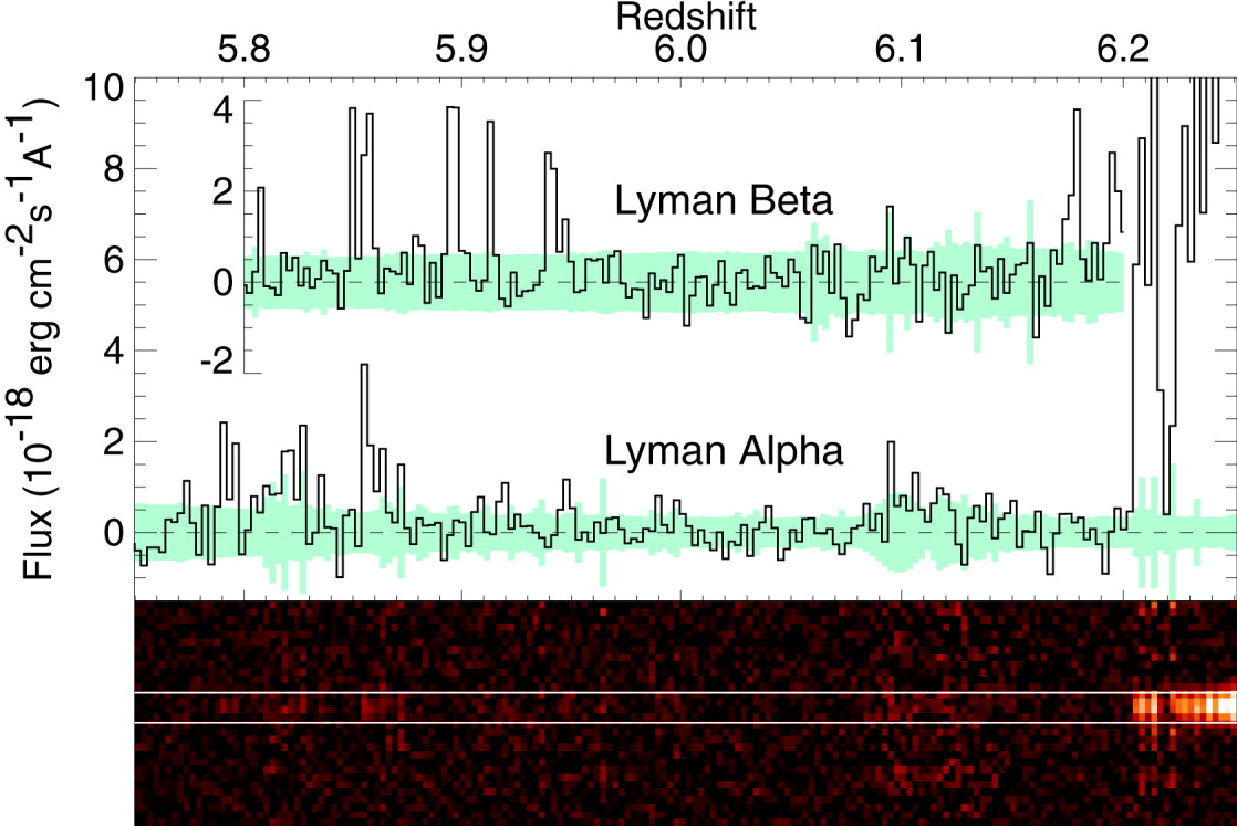
Figure taken from
Becker et al., AJ 122, 285 (2001)
We now think that the hydrogen filling the space between galaxies has undergone two changes since the Big Bang.
It's hard to be specific about the time of re-ionization, since the spectra of different quasars yield somewhat different results. It appears that some regions of the universe may have been more completely re-ionized than others.

Figure taken from
Fan et al., AJ 128, 515 (2004)
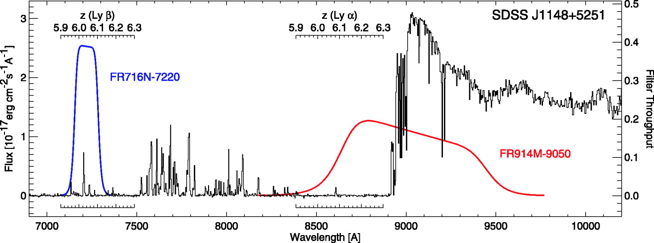
Figure taken from
White et al., AJ 129, 2102 (2005)
The temperature of the CMB in our corner of the universe is currently around 2.7 K.
Image courtesy of
Ned Wright's cosmology site
Now, the Big Bang theory predicts that the temperature of the CMB ought to have been higher in the past. In fact, the temperature ought to rise with redshift in a linear fashion. Is there any way to test this theory? Yes -- but there are two requirements:
Quasars provide the second -- a means to read the thermometer. Let me explain.
The thermometer is provided by several species of atoms or molecules floating in clouds of gas in the interstellar medium; I'll focus on carbon monoxide here. Carbon monoxide, since it is made of two different atoms, has an electric dipole moment. If the dipole spins or vibrates, it will radiate energy rather efficiently. We can detect the radiation emitted or absorbed by the molecule when it makes the transition from one spin (or vibration, or electronic) state to a different one; by comparing the intensity of radiation from several different transitions, we can figure out the populations of the different rotational (or vibrational, or electronic) energy states of the molecules in a gas cloud. In its simplest form, molecules in a cold cloud will all sit in the rotational (or vibrational, or electronic) ground state; a slightly warmer cloud will feature some atoms in the first excited state; a much warmer cloud will feature atoms in the second excited state, and so forth.
The transitions we'll view here are due to molecules which jump from the ground electronic state, n = 1, to the first excited electronic state, n = 2; this corresponds to a large amount of energy, requiring a photon in the near-UV, with wavelength 1544 Angstroms and an energy kTel corresponding to a temperature of order Tel= 20,000 Kelvin. This jump is far beyond the powers of a millimeter-ish CMB photon, of course.
However, the molecules will start and end in different rotational states; these modify the precise energy of the electronic transition by tiny amounts, in which kTrot is of order Trot = 10 Kelvin. Now THAT's small enough for the CMB to have some influence.
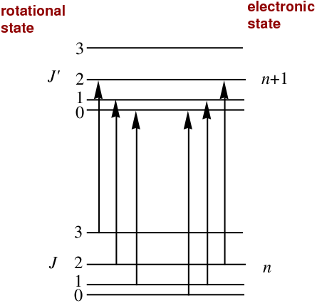
Image courtesy of
Stan Dodds, Rice University
So, the CO molecule will act as our thermometer -- but how can we read it? The emission of light by CO molecules is so weak that it will be swamped by other sources of light.
The key is to use light from a distant quasar as a strong source of continuous radiation; the molecule's absorption of this featureless continuum will tell us about the relative populations of the different energy levels. In other, perhaps fanciful, words, we'll use the shadow of the molecules to reveal their properties.
Let's follow a recent paper by Noterdaeme et al. . They focus on the radiation absorbed in transitions between electronic modes of CO which is in the vibrational ground state, but which may have one of several rotational states. The transitions between electronic states take place in the UV, but can be redshifted to the optical for systems at high redshift. In the example below, you can see the optical absorption lines corrresponding to six different sets of transitions.
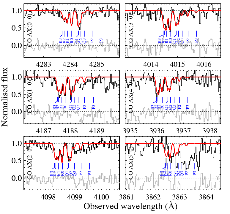
Image taken from
Noterdaeme et al., A&A 526, 7L (2011)
The ratio of the absorption line strengths, together with models of the CO molecule, allow one to deduce the relative number of molecules in the J = 0, 1, 2, and 3 levels (of rotational energy).
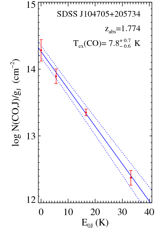
Image taken from
Noterdaeme et al., A&A 526, 7L (2011)
   Q:  What is the most common rotational
       J value for the CO molecules?


   Q:  How many molecules are in the
       J = 0 state for every one molecule
       in the J = 3 state?
Now, the ratios of those levels depends on several factors: the mechanisms for exciting the molecules, and the mechanisms for de-exciting the molecules. A molecule may be kicked up from a low energy to a higher one by a collision with another particle -- that's bad, as it doesn't tell us anything about the CMB -- or it may absorb a photon -- that's good, as the photon might come from the CMB. Ideally, the molecule could only drop down to lower levels due to radiation, as we can measure the rate of those transitions in the lab. In real life, collisions might also cause the molecule to drop to a lower energy state, which would add more variables (density and kinetic energy) to the problem.
Fortunately, in the molecular clouds which host CO molecules, the kinetic temperature of gas particles is low -- around 3 or 4 Kelvin. That means that few collisions can pump a molecule up into the J = 1 or 2 or 3 state. Instead, low-energy microwave photons, such as those from CMB, are the dominant cause of rotational excitation, especially at high redshift. If a quasar just happens to lie behind a cloud of such CO molecules, the UV light it produces may be absorbed by some of the molecules, revealing to careful inspection the exact ratio of molecules in the different rotational states ... which in turn yields the properties of the CMB at that location and time.
In the previous figure, light from the quasar SDSS J104705+205734 shows that a cloud at a redshift of z = 1.774 must be immersed in a CMB with temperature T = 7.8 Kelvin. Noterdaeme et al. measure light from five different quasars, at redshifts ranging from 1.7 to 2.7. The temperatures they derive are shown as red symbols in the graph below; results from other studies, using other molecules or atoms, are in blue or green.
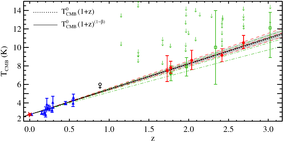
Whoo-hoo! The CMB temperature really does appear to rise linearly with redshift. Maybe this Big Bang theory is a good one ....
When light rays pass through a sufficiently strong gravitational field, they may be deflected slightly. This is the field of gravitational lensing, which has blossomed in the past few decades.

You may have heard of the work by the MACHO , OGLE , and EROS collaborations to search for the gravitational lensing of stars in the LMC (and bulge of the Milky Way) by matter in the halo of the Milky Way. When the lensing mass is of order one solar mass, the term "microlensing" is often used to describe the effect. There are no dramatic changes in size or shape of the background object -- just the brightness. As the lens passes in front of the background object, microlensing produces a light curve of very characteristic shape:
If the lens is not just a single object -- if, say, it consists of a star with a planet nearby -- then the microlensing light curve may become somewhat altered:
Image courtesy of
OGLE collaboration writeup
of a planet detected during the event
OGLE 2003-BLG-235/MOA 2003-BLG-53.
On the other hand, if the lensing object is both very massive and very extended, like a cluster of galaxies, then the background objects can appear magnified, duplicated, stretched out and curved into graceful arcs.

Image of Abell 370 courtesy of
NASA, ESA, the Hubble SM4 ERO Team and ST-ECF
What does all this have to do with quasars? Well, quasars have two (related) properties which turn out to make beautiful music together with the right sort of gravitational lensing:
Suppose we happen to find a quasar lying directly behind some ordinary galaxy. The light from the quasar may be deflected so that we see multiple images of the quasar -- images that are distinct and easy to separate due to Property 1 of quasars.
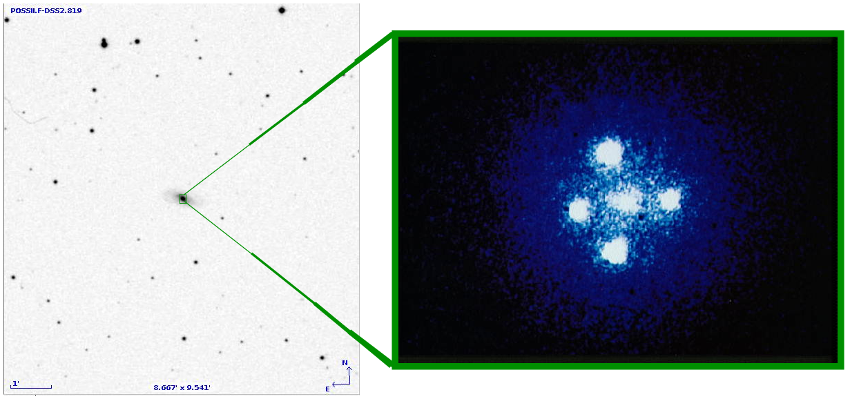
Image of Einstein Cross courtesy of
Johnson Space Center Digital Image Collection
Property 2 of quasars means that we can expect the brightness of each image to change by reasonable amounts -- perhaps 20 percent to 100 percent -- over timescales of days or weeks or months. Moreover, since the light rays for the different images travel different distances along their curved paths to reach us, a single sudden increase in the luminosity of the nucleus will appear to reach us at different times; that is, some of the four images may grow bright long before or long after the others.
The first detection of this effect came in 1997, in the double quasar 0957+561. The two images (A above, B below and close to the nucleus of the lensing galaxy) are separated by a bit more than 6 arcseconds.

Image courtesy of
the Castles group
Can you spot the time delay in these measurements of components A and B, made in the optical g and r passbands?
Figure taken from
Kundic et al., ApJ 482, 75 (1997).
Q: What is the time delay between the two images?
The same system has been measured more recently by Hainline et al., ApJ 744, 104 (2012) . Use their light curves to check your results:
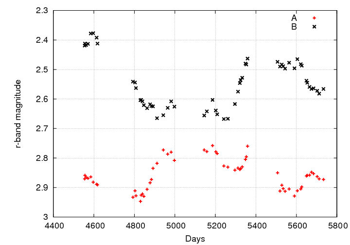
Other systems have since been discovered which offer other chances to measure a time delay between the images in a gravitational lens. For example, the quadruple lens system involving RX J0911.4+0551:
Figure taken from
Hjorth et al., ApJ 572, 11L (2002)
What can you do with this time delay measurement? Well, if you know
it is possible to determine the distance to the lens and to the background source of light. That distance, together with the redshift of the quasar, will yield a nice value of the Hubble constant which is free of many of the systematic uncertainties which plague some other values. Kundic et al. found a value of 51 km/s/Mpc < H0 < 78 km/s/Mpc using their optical data, for example.
Copyright © Michael Richmond.
This work is licensed under a Creative Commons License.