 Copyright © Michael Richmond.
This work is licensed under a Creative Commons License.
Copyright © Michael Richmond.
This work is licensed under a Creative Commons License.
One of the reasons that so many astronomers study galaxy clusters is that they can be used as tools to examine the properties of the universe on scales much larger than themselves. Let's look at several examples.
Ordinary lenses cause light rays to change their direction. If we design them correctly, we can bring different rays to a focus at a desired location.
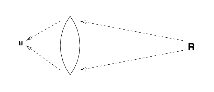
Gravity can cause light rays to change their direction, too.
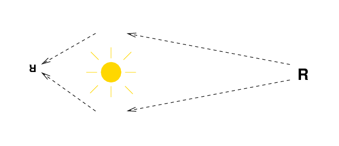
Well, not that dramatically. The deflection of light by gravity is almost always very, very weak. Instead of altering the path of a ray by 10 degrees or even 1 degree, a more typical angle might be just an arcsecond or less. Einstein's famous prediction of the deflection of starlight by the Sun during an eclipse stated that a ray just grazing the photosphere would change its direction by about 1.7 arcseconds.
Clusters of galaxies have lots and lots of mass, so they can act to bend the light rays from background sources. Astronomers often divide lensing into two regimes:

Figure 2 from
Mellier, ARA&A 37, 127 (1999)
A rich galaxy cluster may weakly lens hundreds or thousands of background galaxies; thus, the analysis is dominated by systematics and statistics.
This is what one is hoping to see ...
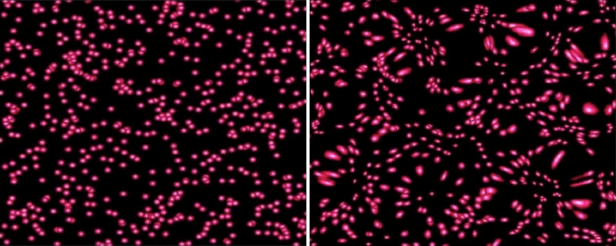
Credit to LSST
and
The Trenches of Discovery
... but one must watch out for nasty systematic errors such as PSF asymmetries.
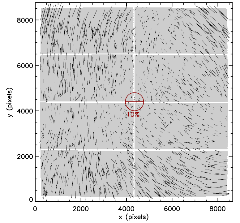
Example of spatial variation in the PSF
at the 4-m Blanco telescope, from
Jee et al., ApJ 765, 74 (2013)
On the other hand, only a few background objects will be located in JUST the right location to be lensed strongly. Good examples are rare, but they offer the opportunity to learn a lot -- including the ability to see objects which would otherwise be invisibly faint. Let's look at a few examples ...
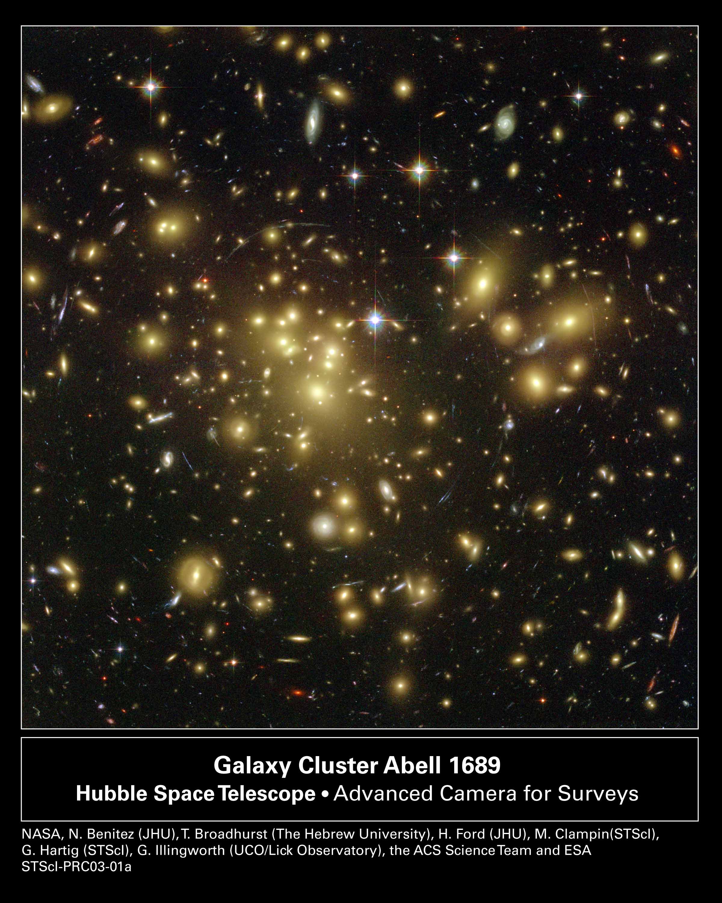
When we look at some rich clusters of galaxies with high spatial resolution, we see long, curved arcs.
The arcs are lensed images of galaxies in the distant background, not part of the cluster itself. In some cases, we see multiple images of a single background galaxy, distorted in different ways as the light rays make their way through the cluster along different lines of sight.
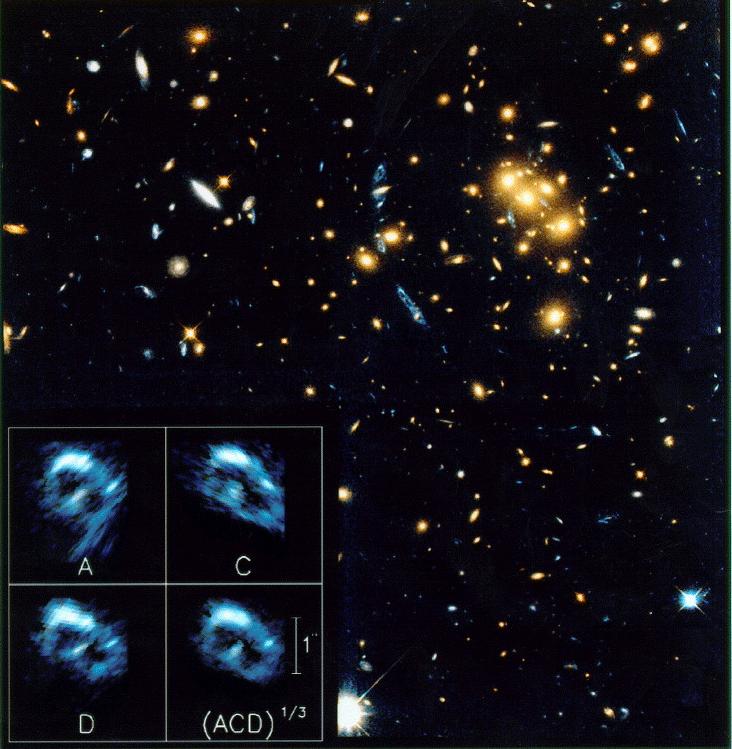
Image courtesy of
Space Telescope Science Institute
If we can discern many details in the lensed images of the background sources, and if we make some simplifying assumptions about the general shape of the matter distribution in the cluster, we can figure out how much matter there must be in the cluster. In other words, we can use the gravitational bending of light to measure the mass in a cluster.
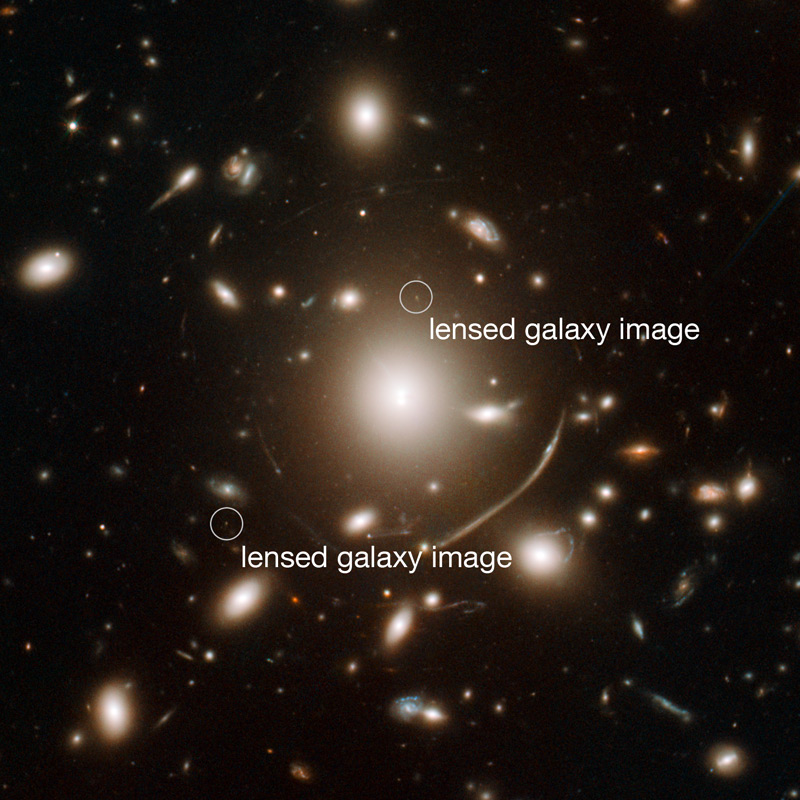
For example, consider this optical image of the cluster Abell 1689.
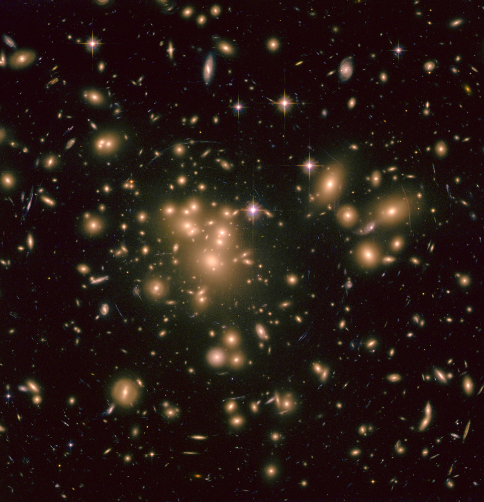
Image courtesy of
NASA, ESA, E. Jullo (Jet Propulsion Laboratory),
P. Natarajan (Yale University),
and J.-P. Kneib (Laboratoire d'Astrophysique de Marseille, CNRS, France)
As described in Coe et al., ApJ 723, 1678 (2010) , one can take the measured positions and brightnesses of galaxies in the cluster itself, the many (over 100) images of background galaxies, together with redshifts for both the cluster and the background galaxies (some determined from spectra, some from colors), and use all that information to make a map of the mass distribution in the cluster. Not just "how much mass?", but the locations and sizes of clumps.
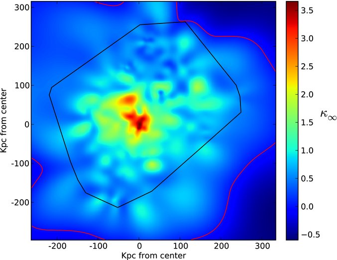
Figure taken from
Coe et al., ApJ 723, 1678 (2010) ,
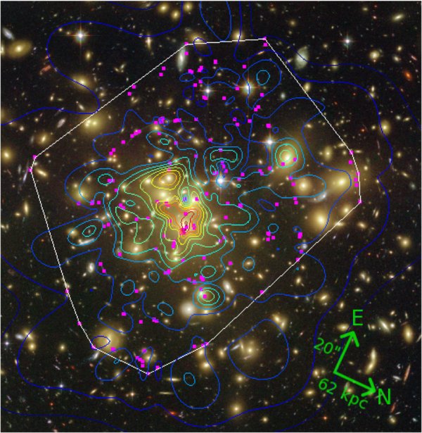
Figure taken from
Coe et al., ApJ 723, 1678 (2010) ,
Here's a slightly more pretty version: the light from galaxies is shown in yellow, the mass based on the model in blue.
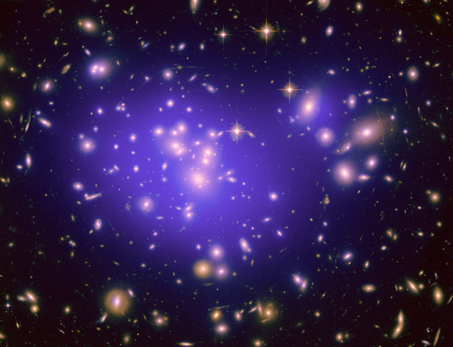
Image courtesy of
NASA, ESA, E. Jullo (JPL), P. Natarajan (Yale), & J.-P. Kneib (LAM, CNRS)
Acknowledgment: H. Ford and N. Benetiz (JHU), & T. Broadhurst (Tel Aviv)
One of the results is a very well constrained model of the mass as a function of radius within the cluster.
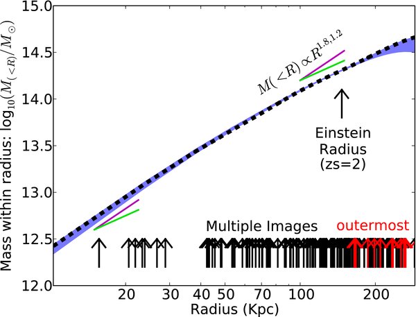
Figure taken from
Coe et al., ApJ 723, 1678 (2010) ,
The authors determine a total mass of the cluster which is roughly 2 x 10¹⁵ solar masses. The mass-to-light ratio for the cluster varies from place to place (now that we have a more detailed map of the mass as well as the light), but it is very high: M/L ~ 200-400 in solar units in places (see Medezinski et al., ApJ 663, 717, 2007, for details).
One can use the gravitational lensing of distant galaxies by clusters as a sort of telescope: the background galaxies will be
In some cases, the good outweighs the bad, and we can take the opportunity to study high-redshift galaxies in much more detail than we could otherwise.
For example, the cluster MS 1358.4+6245 produces images of a number of background galaxies. Pay particular attention to the reddish objects marked with a "1." in the image below.
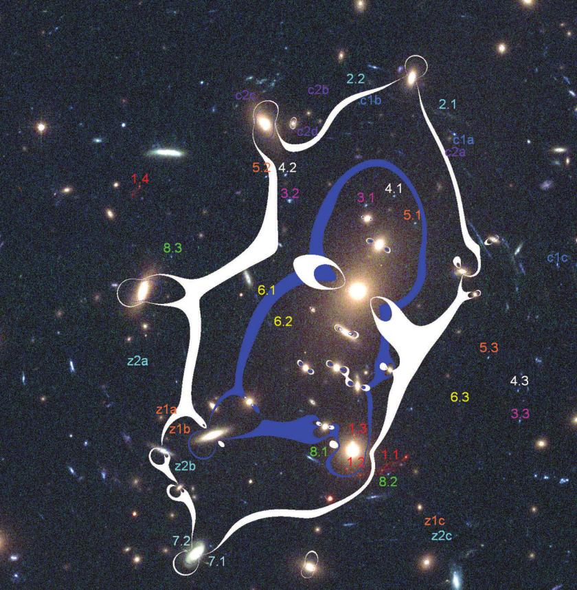
Figure taken from
Zitrin et al., MNRAS in press.
Closeup images of these images reveal differences which are due to the distortion of the gravitational lens. Note that the cluster in this case is NOT a simple spherical or cylindrical mass, but a complex object which creates "caustics" in the lensing plane -- locations at which the background objects are magnified especially strongly.
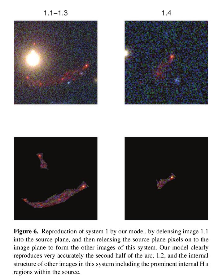
Figure taken from
Zitrin et al., MNRAS in press.
It is possible to reconstruct the original, undistorted appearance of the background galaxy (with some uncertainty, of course). The authors of this study estimate that the lensed image is roughly 80 times brighter than the original would have been. It is also magnified in size: the image you see below shows details which are perhaps 50 pc in size; that's impressive for a galaxy at redshift z = 4.92!
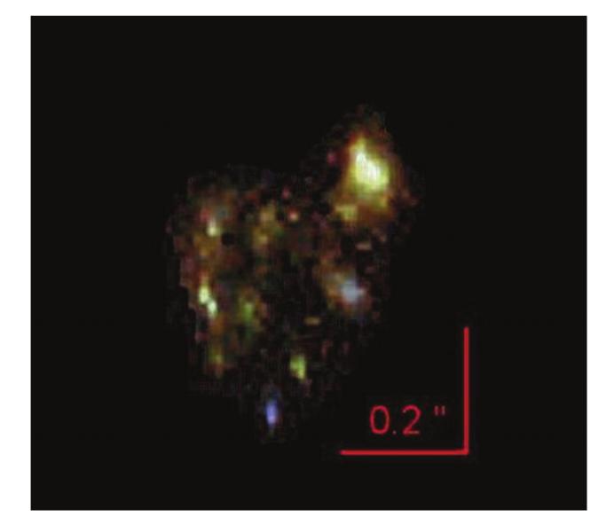
Figure taken from
Zitrin et al., MNRAS in press.
  Q:  A redshift of z = 4.92 corresponds to an
      angular diameter distance of about 1300 Mpc.

      At that distance, what would be the apparent
      angular size of a feature 50 pc in diameter?
      Express your answer in arcseconds.


  Q:  What is the resolution of HST in the optical?
      Use a wavelength of 4000 Angstroms.
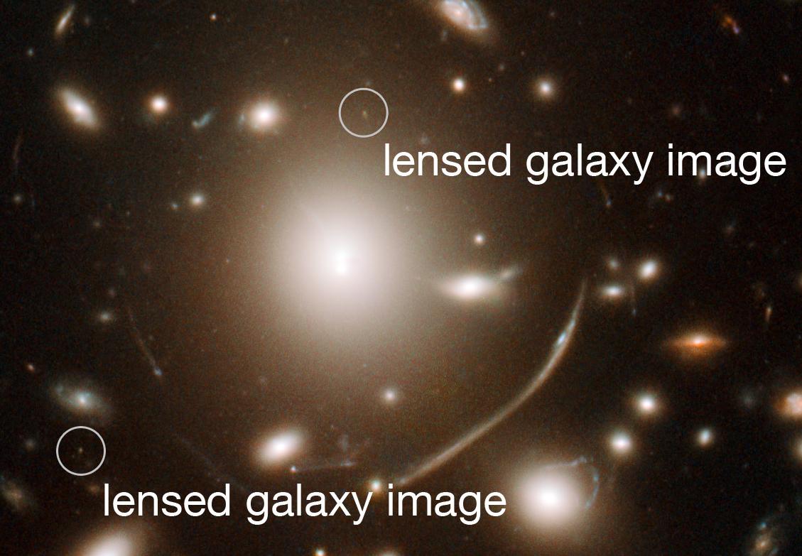
In Dec, 2011, another example of a "cluster telescope" was announced. In this case, the background galaxy was notable for having a particularly high redshift. Judge for yourself. Here's an HST image of the cluster, Abell 383; note the two circled dots.
Clearly, in this case, we can't make out the morphology of the lensed galaxy: it's just a dot. But the lensing has increased the brightness of that background source enough that we can acquire not only magnitudes through several filters, but even a spectrum.
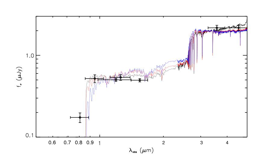
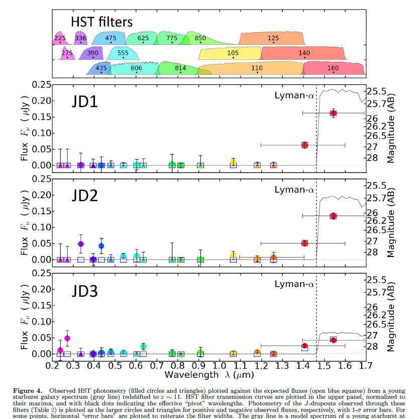
Figure taken from
Richard et al., MNRAS in press
  Q:  There are two steep drops in the model spectra
      shown in the figure above.


      Explain the drop on the right.  What is the
      rest wavelength of this feature?


      Explain the drop on the left.  What is the
      rest wavelength of this feature?


      Based on this fit of a model to the
      photometry, what is the redshift of the galaxy?
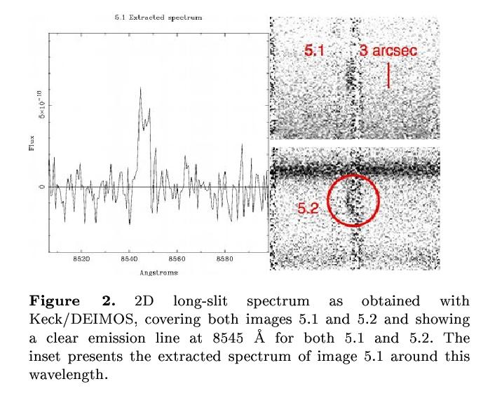
Figure taken from
Richard et al., MNRAS in press
  Q:  The observed wavelength of this emission line
      is 8545 Angstroms.


      What is the claimed identity of this line?


      If true, what is the rest wavelength?


      If true, what is the redshift of this galaxy?
The authors note two aspects of this background source which make it particularly important for cosmological reasons:
Put together, this galaxy places strong constraints in the time during which galaxies may have formed stars after the Big Bang.
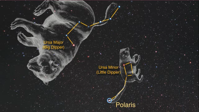
Let's look at another example of a massive cluster of galaxies acting as a "telescope". The cluster known as MACS J0647.7+7015 is not far from the North Celestial Pole, as this pretty movie will show you: click to play.
Coe et al., ApJ 762, 32 (2013) used the strongly distorted arcs and images of background galaxies to make a map of the mass inside the cluster. The picture below shows regions at which the lensing will be particularly strong ("caustics") for background galaxies at different redshifts.

Figure 1 from
Coe et al., ApJ 762, 32 (2013)
The authors noted that three very faint, red objects around the cluster might be images of the same background galaxy.
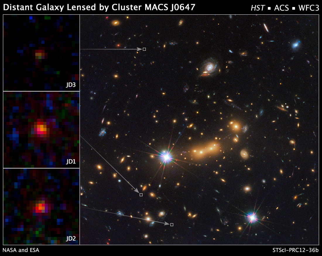
Image taken from
Hubblesite News Release 2012-36
Images taken at different wavelengths showed no emission from the object shorter than about 1.4 microns.
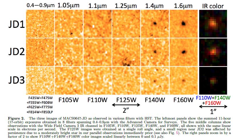
Figure 2 from
Coe et al., ApJ 762, 32 (2013)
Q: Can you estimate the redshift of this object?
You can check your guess by looking at Figure 4 from Coe et al.
Well, a similar thing can happen to photons which pass through the hot gas inside a cluster of galaxies. One source of photons, of course, is the cosmic microwave background.
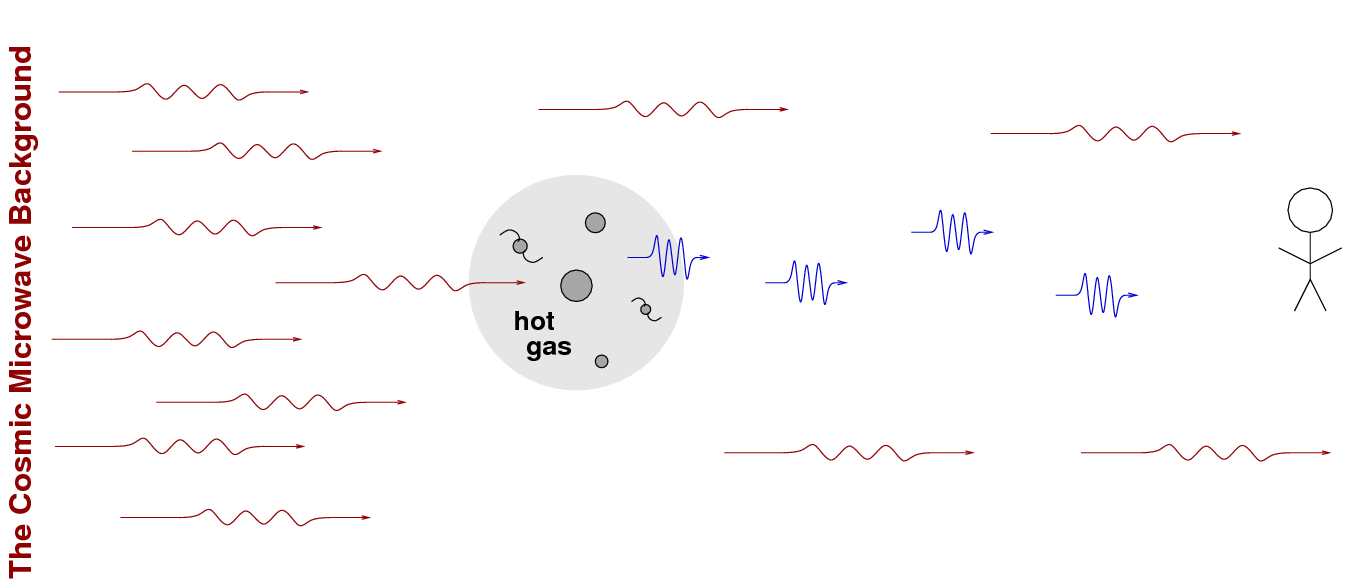
The first treatment of this problem was made by Sunyaev and Zeldovich, ApSS 7, 3 (1970), hence the name.
  Q:  What is the typical temperature of hot gas
      in a rich cluster?


  Q:  How fast are the electrons moving?


  Q:  By what MAXIMUM factor might we expect the energy
      of CMB photons to be boosted?


      (need a hint? look near the end of this lecture)
The result of this inverse Compton shift will be a change in the shape of the CMB spectrum. Overall, photons will move to shorter wavelengths and higher frequencies.
Image courtesy of
Ned Wright's discussion of the SZ effect
Now, the figure above shows a shift which is much, much larger than actually observed. Not every CMB photon will collide with an electron as it travels through the cluster; and those which do interact may not scatter at the ideal angle of 180 degrees (in fact, most will certainly not do so). In real life, the spectrum of the incoming and outgoing CMB is nearly identical. Fortunately, we can use a differential measurement to search for the effect: subtract the spectrum of one location -- say, at the position of a rich cluster -- from a nearby position -- say, several degrees to the side of the cluster. In that case, the SZ effect would produce a difference between the spectra with a pattern like this: a positive difference at higher frequencies (due to the extra high-energy photons at the location of the cluster) and a negative difference at lower frequencies (from which the photons have been "stolen" to create the bump at higher energies).
Image courtesy of
Ned Wright's discussion of the SZ effect
Astronomers have used radio telescopes to search for this effect for some time. The best place to look is near the peak of the spectrum, in the microwaves with wavelengths of a few millimeters. One must use an array of radio telescopes in order to achieve the spatial resolution necessary to resolve (or almost resolve) a distant galaxy cluster. Below is the differential spectrum for the cluster Abell 2163, measured by a collaboration of astronomers using different instruments.
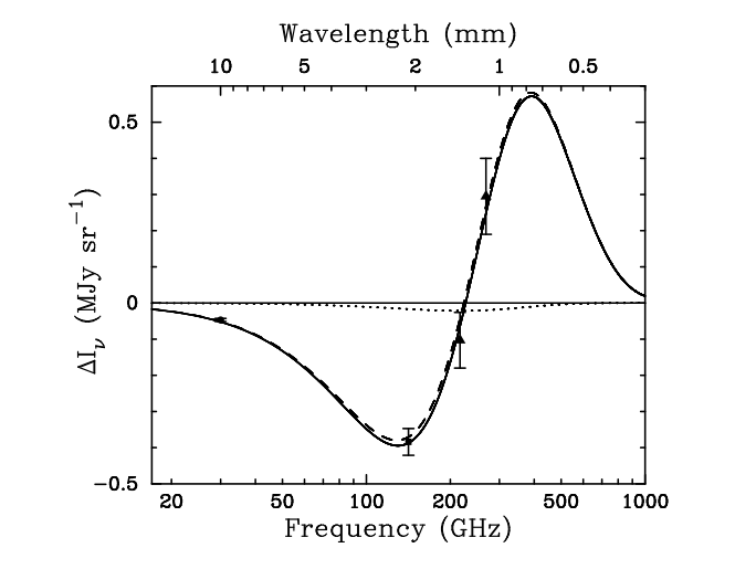
Figure taken from
Carlstrom, Holder and Reese, ARA&A 40, 643 (2002) .
Below are images showing the SZE effect for a sample of clusters at different distances. The color shows the magnitude of the differential SZ effect: red means "large positive difference in spectrum" and black "slightly negative difference". The contours are drawn at multiples of 2-sigma. The white oval at lower left indicates the shape and size of the synthesized radio beam.
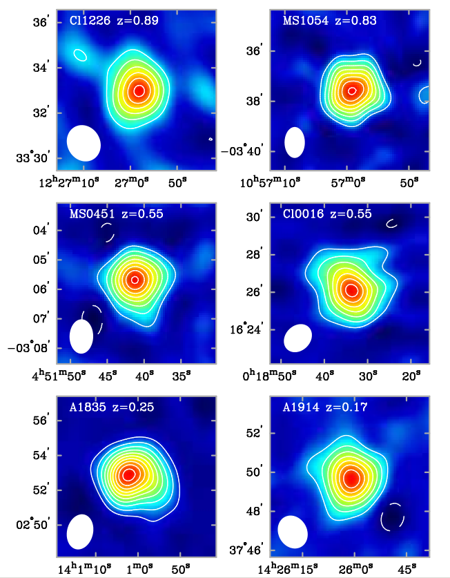
Figure taken from
Carlstrom, Holder and Reese, ARA&A 40, 643 (2002) .
Here's another example of the SZ effect. The upper panel shows the thermal SZ map of the Shapley Supercluster, as measured by the Planck satellite; the lower panel is a composite showing the cluster in optical light (white on black background), X-rays (pink), and the thermal SZ map in the microwave (cyan).

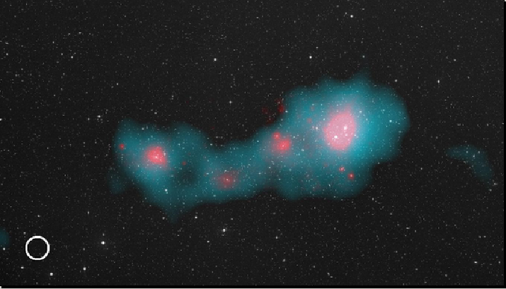
Images taken from
Planck Collaboration XXIX. Planck catalogue of
Sunyaev-Zeldovich sources (2013)
Fine, we can detect the Sunyaev-Zeldovich effect. Is it anything more than a curiosity? What's so great about it? Well, consider these facts:
The SZ effect provides astronomers with a method for finding or confirming the presence of very distant clusters of galaxies; and, with further study, can provide information on the properties of those galaxies. It is a powerful technique, often combined with X-ray observations, which can tell us something about the evolution of structure at high redshift.
Now, this topic isn't strongly associated with galaxy clusters, but I frequently confuse it with the SZ effect, so we might as well discuss it now. Almost fifty years ago, Sachs and Wolfe, ApJ 147, 73 (1967) described what might happen if the universe happened to contain inhomogeneities of mass on very large scales. Cosmic microwave background photons travelling through these concentrations of mass would experience small redshifts or blueshifts; after a very long journey involving encounters with several density fluctuations, the photons might end up with a small change in their energy.
Now, to some extent, the basic idea behind this process involves a symmetry: a photon will gain energy as it falls into a cluster's gravitational potential well, and so become blueshifted; but then, as it flies out of the cluster, it must climb back up that same gravitational well, and so give back the energy it has gained. The net result is no change in energy at all.
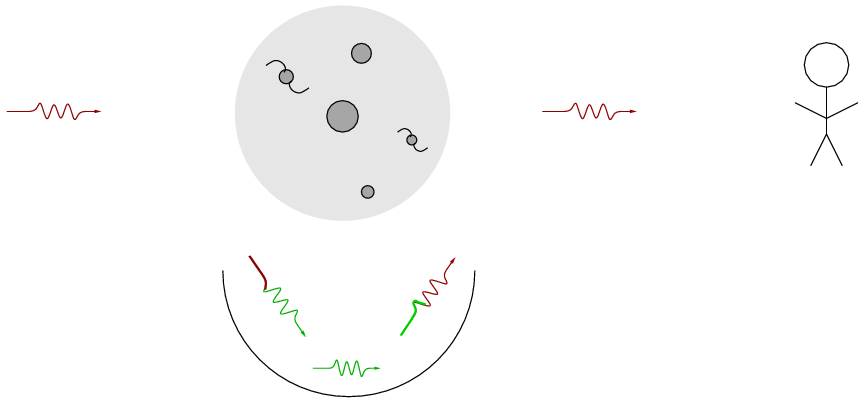
However, if the universe has a non-zero cosmological constant, then the symmetry is broken. Let us consider a VERY large scale concentration of mass -- a supercluster, rather than an ordinary cluster of galaxies. Once again, a CMB photon falls into the gravitational well of the concentrated mass ...

Now, however, during the time it takes the photon to travel through the supercluster, the universe in that region is still expanding due to the effect of the cosmological constant. As a result, the depth of the gravitational well decreases while the photon is inside the well. The photon needs to climb only a small distance to escape the well.

When the photon reaches the Earth, it will have gained a small amount of energy from its trip into and out of the gravitational well of the supercluster. Compared to photons from other regions of the CMB, it will have a slightly higher energy, and a slightly higher frequency. (Click on the figure below to watch an animation)
If my schematic diagrams bore you, you can find
Although the SZ effect and the Sachs-Wolfe effect (or, as it is often called, the ISW = Integrated Sachs-Wolfe effect) both involve boosting the energy of CMB photons by a small amount, they occur on very different scales. The SZ effect is caused by a single cluster of galaxies, which might span a region 1 Mpc in size and subtend an angle (from our point of view) of 3-20 arcminutes. The ISW, on the other hand, requires a region of order tens or hundreds of Mpc, spanning many degrees on the sky.
Another difference is that the SZ effect has been detected and measured for many different clusters of galaxies. The ISW, on the other hand, is still at the stage of being a 5-sigma-ish detection based on cross-correlations of very large datasets. Scientists look for regions of the sky with slightly higher-than-average energies of the CMB, and they look for regions of the sky with slightly higher-than-average numbers of galaxies; if the two sets of regions tend to correlate well with each other, then one can claim that the ISW is responsible.
For example, Granett, Neyrinck and Szapudi, ApJ 683, 99 (2008) choose regions of sky where there are concentrations or anti-concentrations (voids) of galaxies, as measured by the counts of Luminous Red Galaxies in the SDSS. For each cluster (or void), they cut out a little section of a map of the CMB from the WMAP satellite's dataset. After rotating those maps to match the major axis of each cluster (or void), they add all the maps together.
If these clusters (and voids) are really producing an ISW effect, then we ought to see a lower-than-average temperature of the CMB in the direction of voids, and a higher-than-average temperature of the CMB in the direction of clusters.
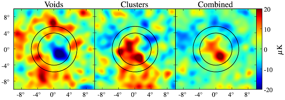
Figure taken from
Granett, Neyrinck and Szapudi, ApJ 683, 99 (2008)
Q: Do you believe?
But wait -- in the five years since the paper by Granett, Neyrinck and Szapudi, astronomers have improved their measurements of the CMB. In March 2013, the results of the Planck mission were released. Let's look at the Sachs-Wolfe effect in stacked Planck data:
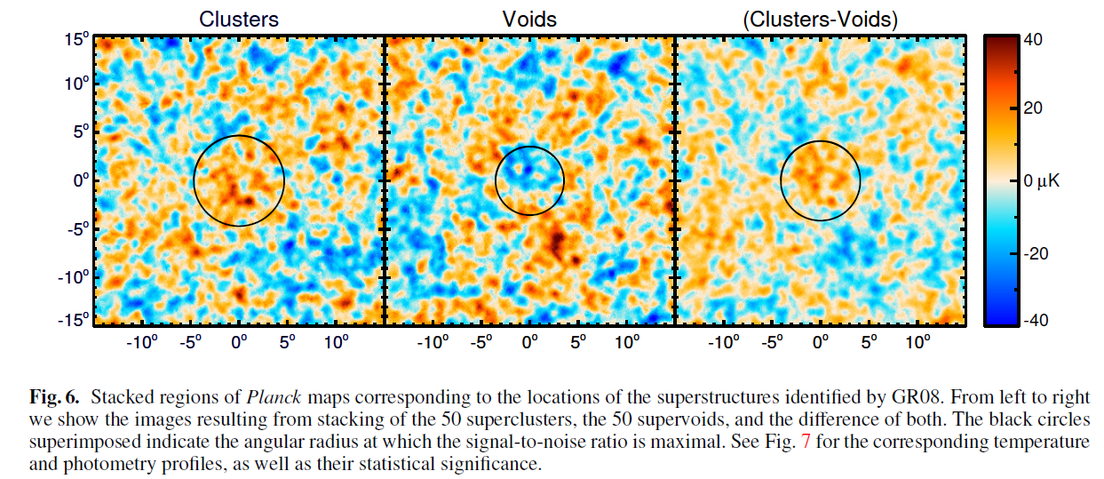
Taken from
Planck 2013 results. XIX. The integrated Sachs-Wolfe effect
Q: Do you believe now?
Copyright © Michael Richmond.
This work is licensed under a Creative Commons License.