 Copyright © Michael Richmond.
This work is licensed under a Creative Commons License.
Copyright © Michael Richmond.
This work is licensed under a Creative Commons License.
We have reached distances so large that all we can see are the bulk properties of entire galaxies; the details are too small to be distinguished, or too faint for us to measure properly. In our previous lecture, we examined the connection between the luminosity of SPIRAL galaxies and the motions of gas within them. Today, we turn our attention to ELLIPTICAL galaxies, which do not, alas, host many clouds of gas. They do, however, contain billions and billions of stars, and so today we look at a relatioship between the luminosity of elliptical galaxies and the motions of the stars within them.
Our story begins in 1976, when astronomers Sandy Faber and Robert Jackson published a paper we will call FJ76. This paper described a set of relationships between some observable properties of elliptical galaxies.
The title begins with the phrase velocity dispersion, so we ought to start by explaining its meaning.
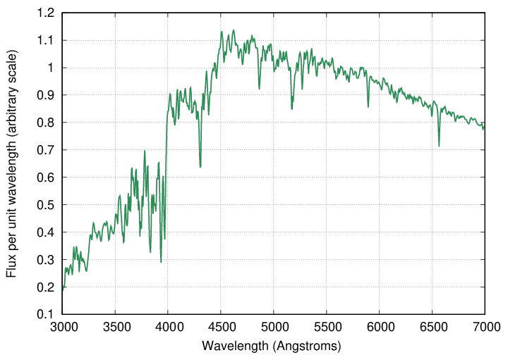
Consider a single, isolated star, motionless relative to us. A spectrum of the star in the optical range will typically look somewhat like this example (which happens to be similar to our Sun): a broad continuum with a number of narrow absorption lines.
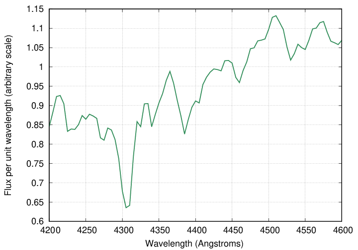
Let's zoom in on a small section of this spectrum in the blue portion of the visible.
Now, if this star happened to moving away from us with speed v, the Doppler effect would shift the wavelength of its lines to the red. The size of this shift is given by
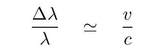
  Q:  If the star were moving away from us at v = 500 km/s,
           how large would the shift in wavelength be?

           At what wavelength would we observe the line in that case?
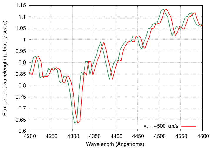
If, for example, we observed a second star, identical to the first but moving at a speed of v = 500 km/s away from us, our measurements of the second star would show its lines shifted like so:
Likewise, if there happened to be a third star, again identical to the first, but this time moving at a speed of v = 500 km/s toward us, its features would appear to be shifted to shorter wavelengths.
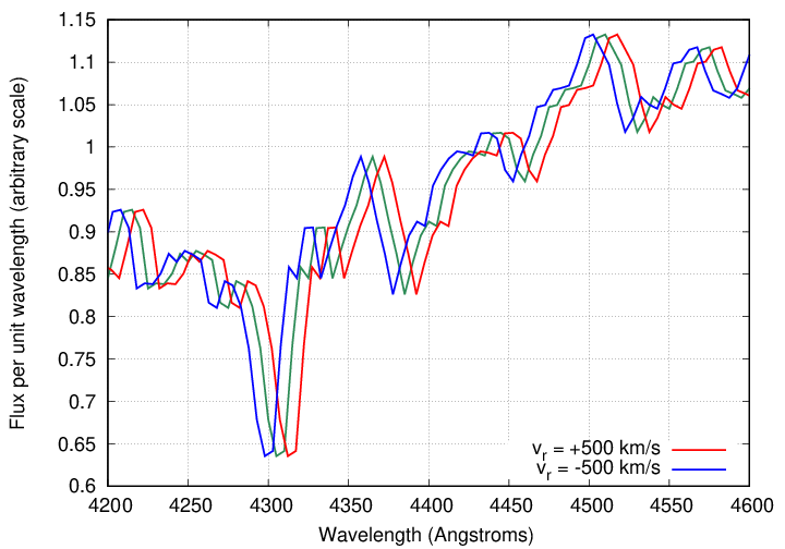
  Q:  If we observed all three stars at the same time,
         so that their light was mixed together,
         in what way would the appearance of this combined
         spectrum differ from the original spectrum of
         the single motionless star?
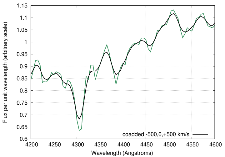
As you can see, the spectrum of a set of stars with a range of radial velocities differs from the spectrum of a single star in two ways:
In other words, the spectral absorption lines become broader and shallower.
In real life, of course, the spectrum of a galaxy is a combination of more than two or three stars; it's a combination of the light of BILLIONS of stars. In a spiral galaxy, since most of the star orbit the center in the same direction, one can describe these motions in terms of a rotation; the speed might depend on the distance from the center, but it's still a pretty simple relationship.
Most elliptical galaxies, on the other hand, do not have a significant rotation; that is, the motions of the stars within them show little evidence for a common direction. However, in some galaxies (which tend to be the massive ones), the stars move very quickly in their orbits; in others (which tend to have small masses), the stars move relatively slowly. One way to quantify the motions of stars in such systems is by the "dispersion" of their velocities: mathematically speaking, if we could measure the radial velocities vi of N individual stars i in a galaxy (which we can't, in almost all cases), the velocity dispersion σ could be calculated as
where ![]() is the average velocity.
is the average velocity.
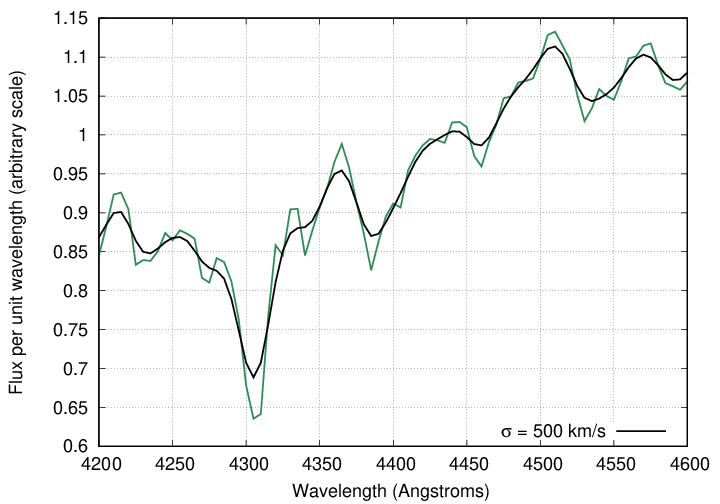
Using a mathematical technique called convolution, one can compute the spectrum of a galaxy in which the stars are moving randomly with any particular velocity dispersion. For example, if σ = 500 km/s, then the spectrum looks like this:
Faber and Jackson measured the velocity dispersion in their sample of elliptical galaxies by comparing the spectrum of light from the center of each galaxy to a series of synthetic spectra, in which a single template spectrum was broadened in a series of steps:
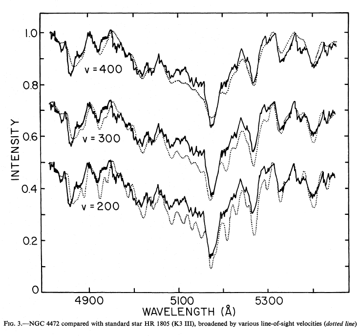
Fig 3 taken from
FJ76.
When they compared the velocity dispersion of each galaxy to the absolute magnitude of the galaxy, they found a pretty good correlation: galaxies with large velocity dispersions tend to be more luminous.
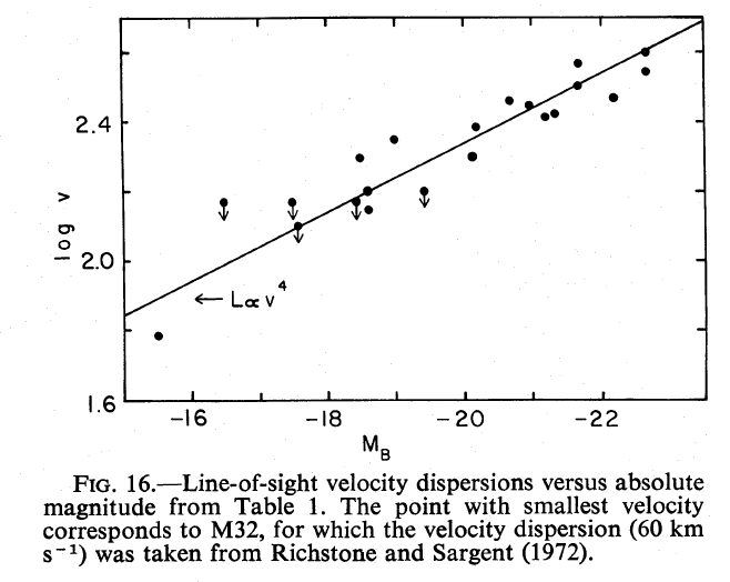
Fig 16 taken from
FJ76.
This correlation between velocity dispersion σ and absolute magnitude (or luminosity) has become known as the Faber-Jackson relation. It ought to remind you of the Tully-Fisher relationship. Perhaps modifying the graph so that its axes are arranged the same way as Tully and Fisher drew them will help. Oh, and I'll add a copy of the graph from TF77, too.
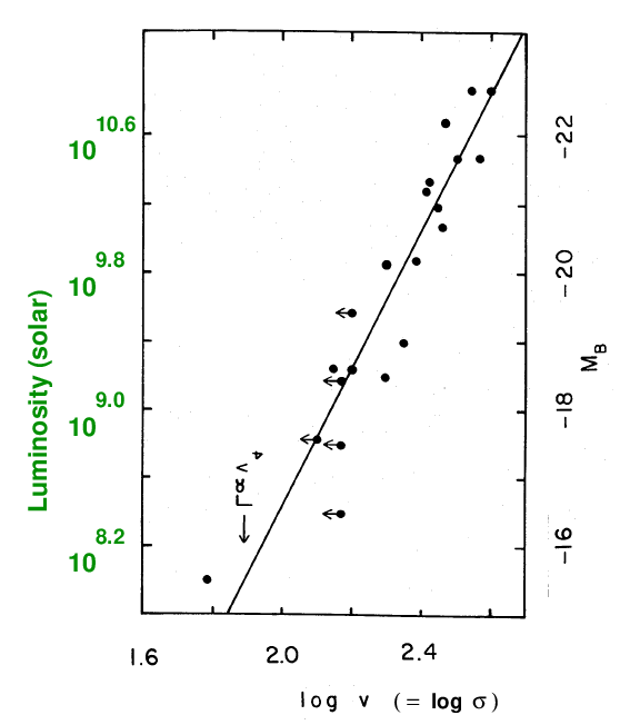
(left) Transmogrified version of Figure 16 from
FJ76.
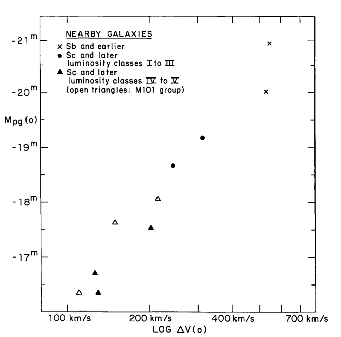
(right) Figure 1 taken from
Tully and Fisher, A&A, 54, 661 (1977)
   Suppose that there is a power-law relationship beween the velocity
       dispersion and luminosity of an elliptical galaxy.
       Use the data on the left-hand panel of the figure above
       to measure the slope of the relationship.

   Q:  What is the exponent of the power law?


                  L  ∝  σ???
In order to apply the Faber-Jackson relationship to estimate the distance to an elliptical galaxy, one can follow this procedure.
Another connection can be made between velocity dispersion and mass-to-light ratio: galaxies with high velocity dispersions also have high mass-to-light ratios. Since velocity dispersion is correlated with absolute magnitude, this means that mass-to-light ratio is also correlated with absolute magnitude.
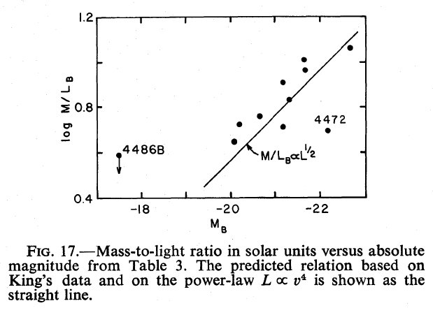
Fig 17 taken from
FJ76.
So, let's summarize the findings of FJ76: elliptical galaxies (*) appear to be a family of objects which are vary in a systematic way, as a function of a single parameter.
(*) aside from dwarf ellipticals
   low mass                                       high mass

   <------------------------------------------------------>

   low luminosity                            high luminosity

   small velocity dispersion       large velocity dispersion

   low mass-to-light ratio          high mass-to-light ratio

   <------------------------------------------------------>
In the years since FJ76, astronomers have accumulated many more observations of elliptical galaxies. We confirm that there is some close connection between several fundamental properties of ordinary elliptical galaxies.
The top-left panel from this figure Diaz and Muriel, MNRAS 364, 1299 (2005) shows a more recent version of the luminosity vs. velocity disperson relationship. It's obvious, but note that there is quite a bit of scatter around the trend. The relationship looks a little bit tighter if one plots luminosity as a function of size, as shown in the panel at top right.
Fig 2 taken from
Diaz and Muriel, MNRAS 364, 1299 (2005)
Now, the bottom-left panel shows a rather weak dependence between velocity dispersion and radius: big galaxies have high velocity dispersions. But there might be some sort of systematic skewing: maybe the connection between radius and velocity dispersion does run exactly along the same lines as the connection between radius and luminosity. In that case, we could improve the quality of the relationship by throwing all three quantities into a big blender -- if we mix them up in JUST the right proportion, we can find a model which matches the observations better than the simple one. Look at the bottom-right panel in the figure above.
Because there are three variables, not just two, people describe this relationship among the properties of elliptical galaxies as the fundamental plane (the term was coined by Djorgovski and Davis in 1987). The idea is that we can use any two of the three quantities to predict the value of the third, in some manner equivalent to:

There are many different ways that one can express this idea, given that each quantity can be described in several different ways, and on scales with may be linear or logarithmic. Bernardi et al,, AJ 125, 1866 (2003) show how the relationship between dynamics, luminosity, and size is seen in passbands across the optical.
Figure 1 taken from
Bernardi et al,, AJ 125, 1866 (2003)
So, how does all of this help us to find the distance to an elliptical galaxy? Well, if we have carefully measured the properties of many galaxies, we may be able to determine the "constant" in the fundamental plane equation,
and so turn it around to solve for the luminosity of a galaxy:
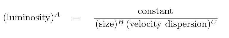
The terms on the right-hand side are both observable quantities, although each must be defined carefully and in a consistant manner. The velocity dispersion is more difficult to measure, requiring a big telescope to measure the spectrum with decent resolution.
How well does it work? A recent paper, Scott et al., MNRAS 451, 2723 (2015), describes measurements of elliptical galaxies in three relatively distant clusters, averaging z = 0.05. The authors find that if they choose the galaxies carefully, limiting the objects to the most luminous examples, and make a particular set of measurements in a particular way, the scatter in the relative luminosities is pretty small:
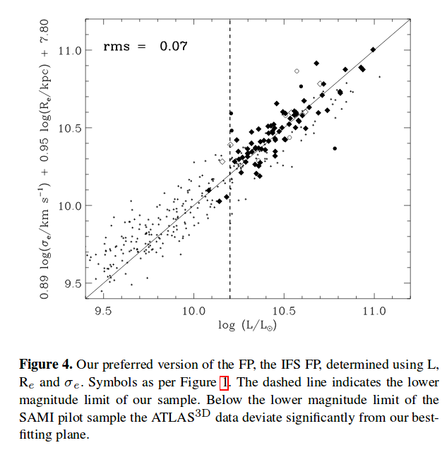
Figure 4 from
Scott et al., MNRAS 451, 2723 (2015)
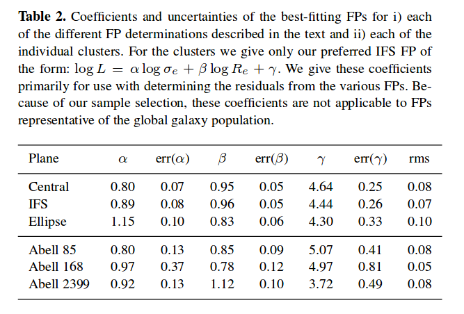
Table 2 from
Scott et al., MNRAS 451, 2723 (2015)
  Q:  Estimate the uncertainty in values of log L from this table.


  Q:  What is the percentage uncertainty in L?


  Q:  What is the percentage uncertainty in relative distances
          computed using such values?
How far away can we use this technique? Well, the good news is that our current instruments can measure these quantities in some elliptical galaxies out to redshifts beyond z = 1.
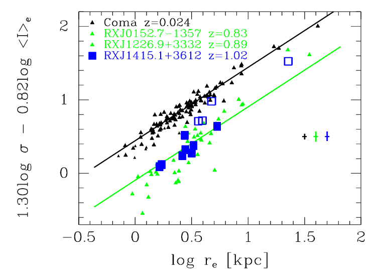
Taken from Figure 2 of
Fritz et al., AN 330, 931 (2009)
The bad news is the same as that for the Tully-Fisher method: at these large distances, we are looking far enough into the past that the stellar populations in the distant galaxies are considerably different from those in local galaxies. Trying to apply this method will involve some complex adjustment for the changing stellar properties, which makes it less reliable.
Copyright © Michael Richmond.
This work is licensed under a Creative Commons License.