 Copyright © Michael Richmond.
This work is licensed under a Creative Commons License.
Copyright © Michael Richmond.
This work is licensed under a Creative Commons License.
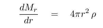
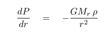
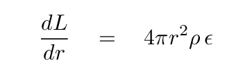
Over the past few lectures, we have derived differential equations for four fundamental properties of a star, all as a function of radius from the center.
And one of the following, depending on whether energy is transported by radiation
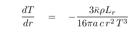
or convection
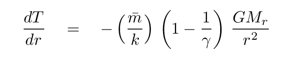
When we build a stellar model, we break the star up into thin little spherical shells, and assume that the properties are constant throughout each shell. Suppose that we have run our model successfully up to shell number 100, and so we know the values in this shell for
Now, these aren't the only quantities which affect the nature of the material in this shell. There are a bunch of others, such as
Q: How can we determine the values of these other quantities?
The answer is, in brief, to use some "equations of state," which describe the relationships between the various properties of a material. For example, in the case of density, we can apply the Ideal Gas Law, which states that
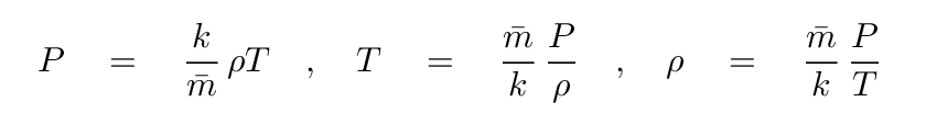
and so compute the density based on the known temperature and pressure.
In order to find the opacity, we need to use some other, and more complicated relationships, as the physical mechanisms by which light and matter interact will change depending on the ionization state and excitation states of the atoms, etc. Fortunately, others have devised both formulae which provide approximate values for these quantities over certain ranges of temperature and pressure, or tables in which one can look up the values for some particular set of conditions. As long as we have access to these auxiliary sources of information, we can use the basic quantities to derive/compute/look up these other properties.
Once we know all the relevant properties of the gas in shell number 100, then we can apply the differential equations to compute the properties in shell number 101. For example, in order to compute the mass interior to shell 101, we could use the very simple Euler's method

Or, if we wished to achieve a higher level of accuracy, we might apply some more complicated technique, such as estimating the values of the derivatives with respect to r at several locations and then applying the fourth-order Runge Kutta method (which is the approproach taken in the STATSTAR program).
The main loop of a program which builds a model of a star would look something like this:
    LOOP:  while not finished

           1. use current values of Mr, Lr, T, P to compute other properties in this shell

           2. calculate derivatives of Mr, Lr, T, P with respect to r

           3. apply derivatives to compute Mr, L, T, P in next shell

           4. move to next shell

           5. go to LOOP
It looks pretty straightforward ... and it IS pretty straightforward, apart from a few tricky bits. Starting the procedure, from either the outermost or innermost shell, requires a number of approximations, and deciding when to end the main loop can also take some thought. Finally, one needs at the end to figure out whether the results MAKE SENSE; as you will see if you try running STATSTAR for yourself, the procedure may very frequently not produce a viable model.
Let us play the part of a computer to see exactly how it works. The star we will simulate is similar to -- but not exactly the same as -- the Sun. These are the properties one can provide as input to the STATSTAR program to reproduce the material shown below.
Q: What is the helium fraction by mass in this star?
Running the STATSTAR program with these input values will yield a valid stellar model. In one of the outer shells, we find the following properties:
In this region of the outer atmosphere, the mass interior to the shell is almost the entire mass of the star. In order to avoid losing precision in computations, the program doesn't tabulate the mass itself, but rather a quantity QM defined as
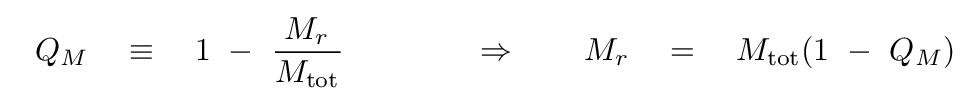
For this shell, this variable has value QM = 3.46 x 10⁻⁹. But in our calculations for this demonstration, we can use the total mass of the star.
  Q:  What is the value of the temperature derivative in this shell?


  Q:  What is the temperature of the next-inner shell?
  Q:  What is the value of the pressure derivative in this shell?


  Q:  What is the pressure of the next-inner shell?
  Q:  What is the value of the luminosity derivative in this shell?


  Q:  What is the luminosity of the next-inner shell?
  Q:  What is the value of the mass derivative in this shell?


  Q:  What is the mass interior to the next-inner shell?
Now, I hope, you have a better idea of how one can build a stellar model inside a computer. If we were to continue doing all the work manually, however, it would take a day or two to run through the several hundred shells that are required to make an accurate model. There was no quicker method back in the Not So Good Ol' Days of the 1930s and 1940s, but we can now give the task of performing all these repetitive calculations to a computer.
The authors of our textbook, Bradley Caroll and Dale Ostlie, provided a computer program in Appendix H which calculates the properties of a stellar model. They call it STATSTAR. It is written in FORTRAN, and you can, if you wish, type in the entire program from their listing. However, it might be quicker to just grab a copy from someone who has done so already.
How does one use this program? When one runs it, the program asks for five items from the input:
The program will compute a set of initial conditions at the outermost layer of the star, then enter a main loop in which it walks inward through the star towards its center. When it reaches one of the ending conditions -- most of which signal a failure of some sort -- it prints a set of diagnostic messages to the standout output. In addition, it writes a list the properties of the calculated stellar model, success or failure, into a text file named starmodl.dat.
As an example, given this sample input file, statstar.in , and running on my Linux system like so:
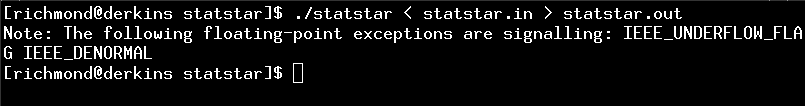
the output file statstar.out is created, holding a brief summary of the results. The full shell-by-shell listing of the model's properties is stored in the file starmodl.dat .
If all goes well, the program will print a message like
               CONGRATULATIONS, I THINK YOU FOUND IT!
         However, be sure to look at your model carefully.
and the output data will be "sensible". What does that mean? It means that the temperature, pressure, etc., will extend from a radius of about zero to a radius of about 1 solar radius (in this case), and each variable will take on appropropriate values at each extreme. For example, temperature should be around 15 million Kelvin at the center, and close to 5000 Kelvin at the outermost shell.
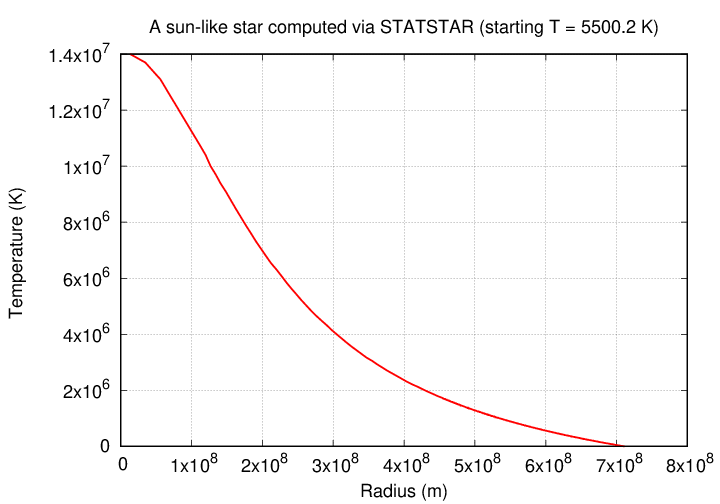
The graph above is an example of a successful run.
But STATSTAR is a simple program, and there is no guarantee that the user's input values will cause the model to reach a "sensible" result by the time the radius decreases to zero. Compare the model which starts at T = 5500 Kelvin to those with temperatures only slightly higher or lower.
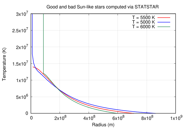
When the starting temperature is higher, the model reaches its target of 1 solar mass before the radius reaches zero -- and the innermost temperature seems to jump up. When the starting temperature is lower, the model again has some issue with the innermost shell.
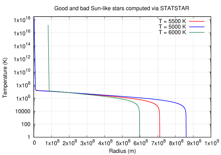
Just how high are those central temperatures? Using a logarithmic y-axis reveals the very ugly truth:
Sometimes the results might look reasonable at first, but upon closer reflection, will reveal that something doesn't add up. If one leaves all the other inputs the same, but decreases the temperature from 5500 to 2000 K, the model is much larger, and may seem okay at first ....
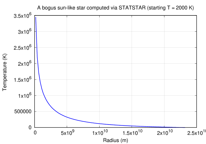
... but look at the central temperature: about 3.5 million K. No significant fusion will take place at such a temperature, and so very little luminosity will be produced, which invalidates the assumption of a roughly solar luminosity.
Although a single run of the program might not produce a good stellar model, one can examine the results, modify the inputs, run again, and continue to adjust the input parameters until the results are consistent. That iterative process might take some time, but not as long as it did back when the program was first written. In the 1996 edition of their book, the authors write:
STATSTAR execution times vary depending on the machine being used. For instance, on PCs with 486 33 MHz chips or higher, a model can be completed in a few seconds; on faster machines only a fraction of a second is required.
A quick test on my home computer shows that the program takes about 2 milliseconds to run a single model.
So we can build models in a computer, but do those models look anything like real stars? If not, the models are good for nothing but wasting CPU cycles. Well, to find out, let's look at one particular set of models, as shown in Iben (ARA&A 5, 571 (1967); in all of these models, the core of the star is fusing hydrogen into helium. The star begins its life at the small symbol labelled with its mass, and then evolves with time up and to the right, following the lines.
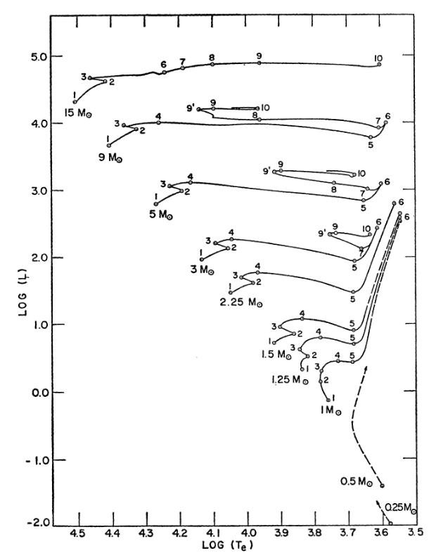
Figure 3 taken from
Iben, ARA&A 5, 571 (1967)
Q: Does these models resemble real stars in their properties?
I think so.
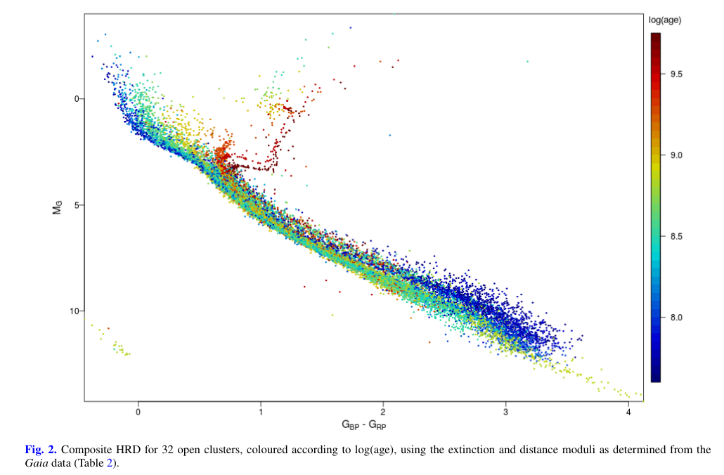
Fig 2, based on Gaia data, from
Gaia Collaboration, A&A 616, A10 (2018)
It tells us, among other things, that stars on the main sequence are fusing hydrogen into helium in their cores.
But that's not all. We can learn more from these models. Consider, for example, the SIZE of stars. Look at the diagram below; in particular, at the stars with masses of 1, 3, and 15 solar masses.
Figure 3 taken from
Iben, ARA&A 5, 571 (1967)
  Q:  Write down the temperature and luminosity of the stars with masses
              1, 3, and 15 times that of the Sun.


  Q:  If the luminosity varies with temperature to some power, like

                   L  =  K Tp

          what is the value of exponent p?
          (Hint: look at the change in log(L) vs. change in log(T)).


  Q:  If stars were constant in size, and differed only in
          temperture, what would the exponent p be?
The luminosity of stars on the main sequence does not change exactly as temperature to the fourth power ... but it's not all that different. Since the luminosity increases as a slightly larger power, stars must grow slightly larger with mass. But not by a huge factor.
       As mass increases from            0.08 M(solar)    to   90 M(solar)

       radius increases from approx      0.1                   20
Note how well lines of constant radius show the same-ish behavior as real stars in the HR diagram.
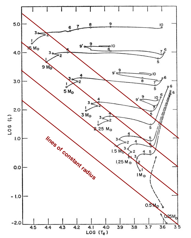
Figure 3 taken from
Iben, ARA&A 5, 571 (1967) ,
with annotations added
Another aspect of stars that these models illuminate is their main sequence lifetime. Ignore all the time-dependent evolution of stars in these models -- just look at the initial positions of stars, at age zero.
    As mass increases from            0.08    M(solar)   to         90 M(solar)

luminosity increases from approx      0.0005  L(solar)       1,000,000 L(solar)


			  Q:  If luminosity depends on mass to some power,


                     L  =  K Mq


               what is the approximate value of the exponent q?
The fact that luminosity on the main sequence increases so rapidly with mass has profound implications for the lifetime of a star on the main sequence. We can compute an approximate lifetime via the simple formula
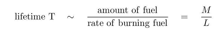
  Q:  Given your relationship between L and M derived a moment ago,
          can you derive an equation relating the main-sequence lifetime
          of a star to its initial mass?
We estimated in a previous lecture that the Sun could continue to burn hydrogen at its current rate for very roughly 10 billion years. Let's use this as a yardstick.
  Q:  Estimate the main-sequence lifetime of a star with  3 solar masses.

  Q:  Estimate the main-sequence lifetime of a star with 10 solar masses.

  Q:  Estimate the main-sequence lifetime of a star with 30 solar masses.
The most massive stars certainly don't last very long. It might be interesting to consider the time it takes for planets to form around a newly-born star ... or the time it takes for life to evolve on a planet ...
Copyright © Michael Richmond.
This work is licensed under a Creative Commons License.