 Copyright © Michael Richmond.
This work is licensed under a Creative Commons License.
Copyright © Michael Richmond.
This work is licensed under a Creative Commons License.
Looking through Earth's atmosphere (in general)
Electromagnetic waves from all sorts of celestial sources fall upon the Earth from all directions, all the time. We have instruments that can detect them over a very wide range of wavelengths:
10-19 meters to 102 meters
That's 21 powers of 10, or, in other words, 21 decades. A huge range, providing information from all sorts of sources.
Unfortunately, when this wealth of information hits the Earth's atmosphere, only a small fraction makes it to the surface.
![]()
Q: How many decades of electromagnetic waves reach the surface?
![]()
Here's another way to look at the effects of the Earth's atmosphere. Note that while high-energy (UV, X-ray and gamma-ray) photons can't reach the ground, they DO penetrate far enough that a balloon-borne instrument might detect them.
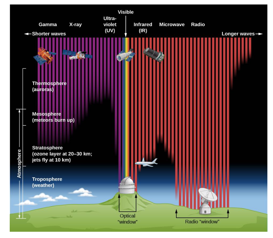
Image courtesy of
OpenStax, Rice University, modification of work by STScI/JHU/NASA
For example, if one is interested in the ultraviolet portion of the spectrum, a balloon at an altitude of 34 km (112,000 feet) can observe nearly half of the incoming photons.
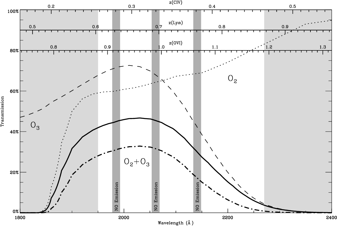
Figure 3.2.1 taken from
Matuszewski, M. K., Ph.D. thesis (2012)
Let's ignore the high-energy ranges that are stopped completely by the Earth's atmosphere (and a good thing, too), and concentrate on the "interesting" regions for ground-based observers. There are two wavelength regimes which we can see from the ground: optical/near-IR, and radio.
![]()
Earth's atmosphere in optical and IR: extinction
We can zoom in even more to examine the regions of the optical and near-infrared -- which are the places I almost always work myself. This is a pretty narrow window: it covers just about 2 decades.
![]()
  Q:  How much of this region belongs to the visible --
         the portion we can see with our own eyes?
That's right: very little. Our eyes can barely detect light spanning a single octave (a factor of two in wavelength), let alone a decade (a factor of ten). The limits of human vision are very roughly
         3500      -     8000     Angstroms

          350             800     nm

         violet           red
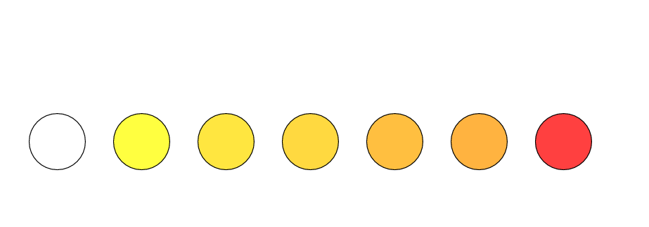
The near-infrared covers a much larger region, from where our eyes stop in the red -- around 8000 Angstroms = 0.8 microns -- to something around 20 or 25 microns. As you can see, the atmosphere does absorb slices of this range, letting only narrow bands pass. Water vapor is responsible for much of this absorption.
Astronomers have labelled the mini-windows within the near-infrared with a set of letters, increasing in (almost) alphabetical order from short wavelengths to long. These letters are also used to describe the filters astronomers use to replicate these regions. So, for example, the Hubble Space Telescope, far above the atmosphere, can use a filter (F125W) which approximates the "J-band".
![]()
Now, even though light can MOSTLY pass through the Earth's atmosphere in the optical and near-IR, some of it is scattered or absorbed by molecules and particles in the air. You are already familiar with some of the consequences of this effect.
For example, when the Sun is high in the sky, so that its light comes nearly straight down through the air, it looks yellowish-white ...

Image courtesy of Jen Connelly
... but when the Sun is low in the sky, so that its light rays must pass through a long stretch of the Earth's atmosphere, it appears orangey-red:
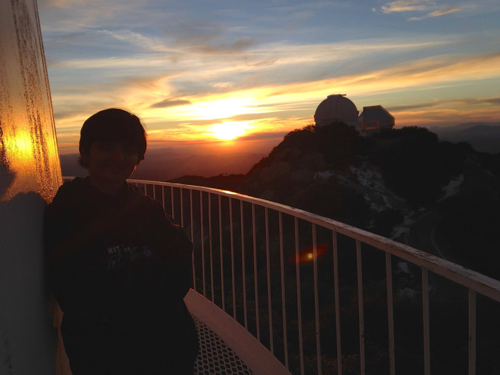
Image courtesy of Jen Connelly
In order to make quantitative estimates of the amount of light which is scattered as rays journey through the atmosphere, we need to figure out the length of their path through the air: more air means more scattering. However, calculating the length of a straight line passing through a circular shell at an arbitrary angle is pretty difficult.
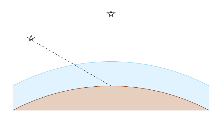
Astronomers have decided that approximating the real, curved surface of the Earth, and volume of the atmosphere, with simple, flat shapes, yields results which are good enough for many purposes.
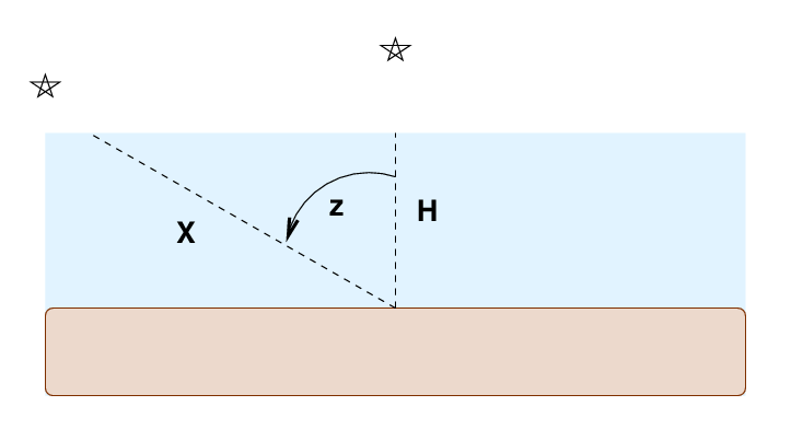
The shortest path, for a star which is directly overhead, has some length H. Astronomers call this minimum distance one air mass. The distance X travelled by a light ray at a zenith angle z is longer ... by how much?
  Q:  Can you write a formula which gives the distance X
        in terms of angle z and H?
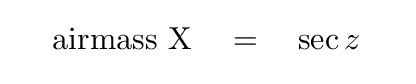
Yes, that's right:
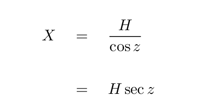
But since we define the minimum distance H as "one airmass", the equation becomes even simpler:
Now, as light travels through the air, it is progressively scattered and absorbed; the farther it goes, the weaker the remaining beam becomes. If we chose to measure the intensity of the light, we would find an exponential relationship between the surviving beam and the airmass, where f is some value that depends on the wavelength of the light.
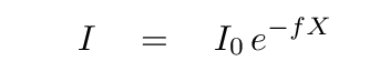
However, if we choose to measure the beam of light in magnitude units, then the relationship between the original brightness, the surviving brightness, and the airmass is a simple linear one:
  Q:  Why does using magnitudes turn the exponential relationship
          into a linear one?


  Q:  What is the relationship between the coefficients f and k?
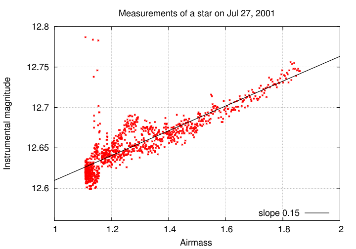
Let's check to see if this approximation really makes sense. On the night of July 27, 2001 , I spent many hours staring at a single region of the sky, making measurements of the variable star WZ Sge. The table below contains measurements of the brightness of a nearby star -- one that does not vary in brightness intrinsically -- as it rose and set. The format of this ASCII text file is something like this:
# Measurements of a bright star in CCD images taken at RIT Obs
#   on July 27, 2001
#   see http://spiff.rit.edu/richmond/ritobs/jul27_2001/jul27_2001.html
#
#airmass                                           instr_mag
1.556       59      1 0    -1 -1.00 -1.00  99.00    12.701  62500
1.554       59      2 0    -1 -1.00 -1.00  99.00    12.704  62500
so the airmass is located in column 1, and the instrumental magnitude of the star in column 9.
   a)  make a graph which shows airmass on the horizontal axis,
           and instrumental magnitude on the vertical axis

   b)  use your graph to estimate the linear coefficient k
           for the extinction in these measurements
My results are shown below.
Now, the constant k in the formula for magnitude as a function of airmass depends on the wavelength of the light:
Optical astronomers use a number of different photometric systems, but one of the most widespread is a set of broad-band bandpasses called the "Johnson" or "Johnson-Cousins" system. Going from blue to red, the passbands are called U, B, V, R, I:
The exact values for the extinction coefficient vary from night to night, and from one location to another, but rough average values are:
   passband         k
 ----------------------
      U            0.6
      B            0.4
      V            0.2
      R            0.1
      I            0.08
  Q:  Which filter was I using at the RIT Observatory on
        July 27, 2001?
You can check you guess here.
Looking through the ISM (in general)
Even if we place a telescope far above the Earth's atmosphere, we still can't see distant objects perfectly. In the vast expanses of space between those sources and our instruments lie atoms and molecules and teeny-tiny particles of dust. Interstellar space is a darn good vacuum -- but it is not a PERFECT vacuum. Given a long enough journey, a light ray will encounter enough stuff that it may be scattered or absorbed.
The graph below gives a rough idea of the regions of the electromagnetic spectrum most affected by the interstellar medium. The most vulnerable photons are soft X-rays, UV, visible, and the near-IR. Photons in the extremes of the electromagnetic spectrum -- gamma-rays and radio waves -- are (for the most part) able to travel freely through space.
ISM in optical/IR: extinction and reddening
Because so many astronomers observe in the optical and near-IR, and because the ISM can contaminate so strongly in these regions, we have devised some rather complicated techniques to detect and remove the effects of dust and gas. I'll provide just a brief introduction to some of them here.
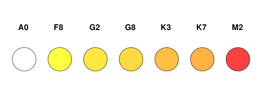
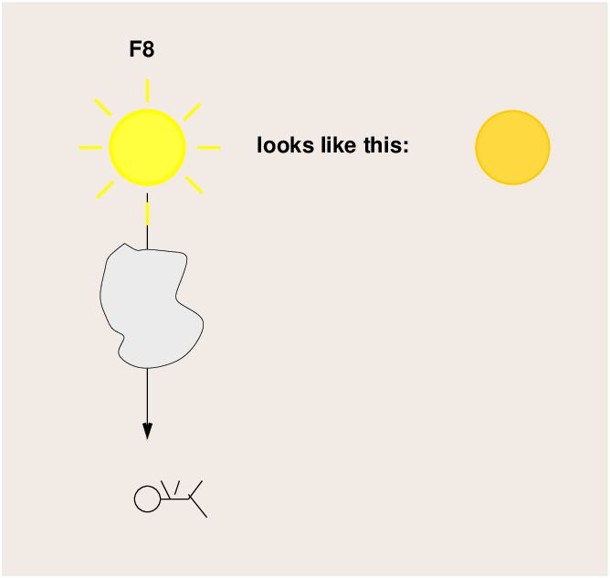
Let's begin by reviewing the properties of ordinary, main-sequence stars. Massive stars have very hot photospheres, and so appear blueish-white; sun-like stars are cooler, and so seem yellowish-white to our eyes; and the coolest dwarfs, at only about 3000 Kelvin, appear reddish.
If we measure the spectra of these stars, we find a wide range of absorption line features which are correlated to the temperature of the photosphere. Astronomers have devised a spectral classification system which attaches labels to stars: each label is connected to a star's temperature through the pattern of the strongest lines.
If we observe these stars through the standard broad-band astronomical filters, such as UBVRI, we will see a systematic change in the apparent magnitudes of stars with their temperature. Consider the B and V filters, for example.
Hot stars will put more light into the blue filters. That means that
The star below might yield B = 1.0 and V = 1.5, so that the color of the star would be (B-V) = 1.0 - 1.5 = -0.5
Cool stars will put more light into the red filters. That means that
The star below might yield B = 5.0 and V = 4.1, so that the color of the star would be (B-V) = 5.0 - 4.1 = +0.9
One can make a table which connects the spectral type of stars to their intrinsic colors; the subscript 0, as in (B-V)0, means "intrinsic to the star, as if observed through a perfect vaccuum." Below is an abbreviated version of one given in Allen's Astrophysical Quantities, Section 99. Please write these down.
  Spectral Type       (B - V)0
 ------------------------------
     B0                 -0.31

     A0                  0.00

     F0                 +0.27

     G0                 +0.58

     K0                 +0.89

     M0                 +1.45
 ------------------------------
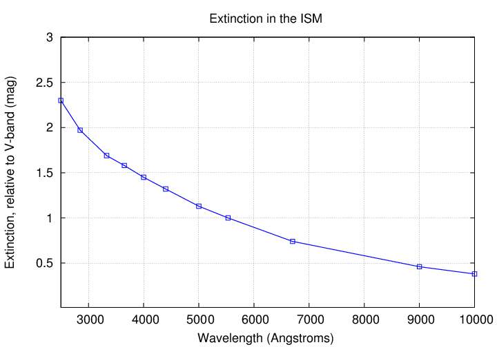
But when light from a star travels through a dust cloud, it will be both extinguished (made fainter overall) and reddened (made more fainter at short wavelengths). Optical astronomers use different symbols to denote these changes.
Extinction is labelled with a capital letter "A", plus a subscript for the passband in question. For example, AV refers to the amount of extinction in the V-band (in magnitudes).
  Q:  Along one particular line of sight, the extinction in the
         V-band (at 5500 Angstroms) is 1.0 magnitudes.
         Use the graph below to estimate the extinction
         in other passbands:

           U-band         3400 Angstroms      AU = __________

           B-band         4400 Angstroms      AB = __________

           I-band         8000 Angstroms      AI = __________
Now, if light from a star happens to fly through a cloud on its way to the Earth, we will see a version of the star which is both REDDER and FAINTER than it ought to be:
If we have three pieces of information, we can determine the amount of both reddening and extinction, and correct for it! Here's what we need:
I'll make up some values in the following discussion to provide a concrete example. You might following along using a simple worksheet.
First, we compute the OBSERVED color of the star, based on the measured magnitudes.
    This star has measured magnitudes of

               B  =  12.90

               V  =  12.00

     The star's measured color is (B-V)  =  ___________
Second, we look up the INTRINSIC color of the star, based on its spectral type.
This star is F0. Its intrinsic color (B-V)0 is: _________
Third, we use the observed and intrinsic colors of the star to calculate its color excess E(B-V) (also known as "reddening") like so:
     color excess  E(B-V)  =   (B-V)  -  (B-V)0

                           =    ______________
How thick must the interstellar cloud be to produce this change in color? Well, could the cloud be so thick that it extinguishes the star by exactly 1.0 magnitudes in V-band?
   If the cloud were just the right thickness to yield AV = 1.0,
      what would the extinction be in B-band, AB?


   In that case, what would the true B-band magnitude be?

   In that case, what would the true V-band magnitude be?

   In that case, what would the true (B-V) color be?
Whoops. Nope. A cloud of that thickness would not produce the amount of reddening that we observe. We must be looking through a thicker cloud ...
Q: Can you figure out the true extinction due to the cloud?
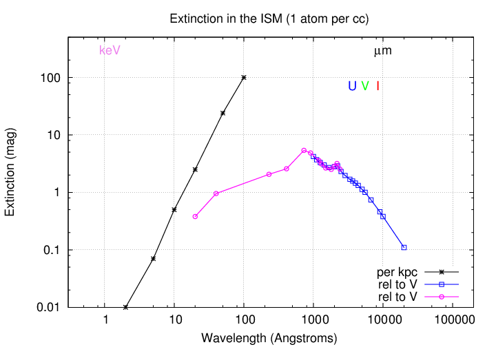
Over the years, astronomers have come up with some quick ways to perform this sort of correction. We begin with a model for the extinction of light by dust and gas, something like that curve you saw earlier:
Based on this sort of model, one can write down the relative amounts of extinction for light in different passbands.
The values below are very rough estimates, read by eye from the graph above. Please consult good reference materials for more accurate values
       passband             extinction (mag)
 -----------------------------------------------
         U                      1.6

         B                      1.33

         V                      1.0

         I                      0.5
 -----------------------------------------------
One can then compute the reddening due to some standard level of extinction. For example, for 1.0 magnitudes of extinction in V-band, we should see AB = 1.33 and AV = 1.0, so
reddening AB - AV = E(B-V) = 0.33
And we can then use the reddening E(B-V) of a star
to compute the extinction in some band,
because the SHAPE of the extinction curve
tells us the ratio of reddening to extinction.
For "typical" clouds in in the interstellar medium,
                              1.0
            AV  =  E(B-V) *  -----  =  E(B-V) * 3.1
                              0.33

                              1.6
            AU  =  E(B-V) *  -----  =  E(B-V) * 5.0
                              0.33

                              1.33
            AB  =  E(B-V) *  -----  =  E(B-V) * 4.1
                              0.33

                              0.5
            AI  =  E(B-V) *  -----  =  E(B-V) * 1.6
                              0.33
In our example above, the reddening of our star was E(B-V) = 0.63, so we can figure out the extinction:
            AV  =  E(B-V) * 3.1  =  0.63 * 3.1  =  1.95 mag

            AB  =  E(B-V) * 4.1  =  0.63 * 4.1  =  2.58 mag

     etc.
In the radio regime, we don't often worry about extinction or reddening; but there is a very different effect that the interstellar medium exerts on radio waves.
Q: Do all radio waves travel at the same speed?
In a vacuum, the answer is "Yes". But in a region filled with charged particles, the answer is "No!" If a radio wave moves through a sea of charged particles, its oscillating electric field will interact with the charges, causing them to oscillate, too. The strength of this interaction depends on several properties; for our purposes, the most important is the FREQUENCY of the wave. The lower the frequency, the stronger the interaction, and the slower the wave propagates. This phenomenon is called dispersion.
I'm no expert on this subject, so please visit real experts to learn about it:
We don't normally worry about this in the optical or infrared or X-ray regimes, because the effect is too small to measure at such high frequencies. In the radio, though, the differences in speed between several wavelengths can be large enough for us to measure.
You've heard of fast radio bursts, right? These mysterious quick little signals are a hot topic for discussion right now, as people try to figure out what they are, and where they are. In January, 2017, one FRB was pinned down to exist (probably) within a not-too-distant galaxy: The direct localization of a fast radio burst and its host by Chatterjee et al., Nature 541, 58 (2017). We think that the source produces a brief burst of radio waves of many frequencies, all at the same time ... but look at the observed signal:
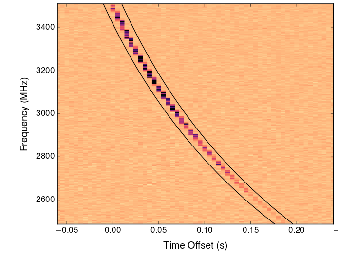
Taken from Figure 1 of
Chatterjee et al., Nature 541, 58 (2017)
Actually, this frequency-dependent delay in the arrival of radio waves can be viewed as a benefit, rather than an annoyance. If the large-scale properties of the ISM are relatively uniform, then the size of this dispersion should depend on the distance between us and the source: more distant sources will suffer larger dispersion. If we know enough about the interstellar medium, we can even use the dispersion of radio waves to estimate distances!
Another result of the interaction between radio waves and the ISM is the "pulse broadening" caused by scattering of waves as they move through an inhomogenous medium. If a wave moves past little blobs of charged particles, portions of it may be refracted just a bit, this way and that way. If there are many little blobs, and many small scatterings, then even waves of a single wavelength may be delayed a bit relative to others. Since low-frequency radio waves interact more strongly with the ISM than high-frequency ones, this effect is strongest at low frequencies.
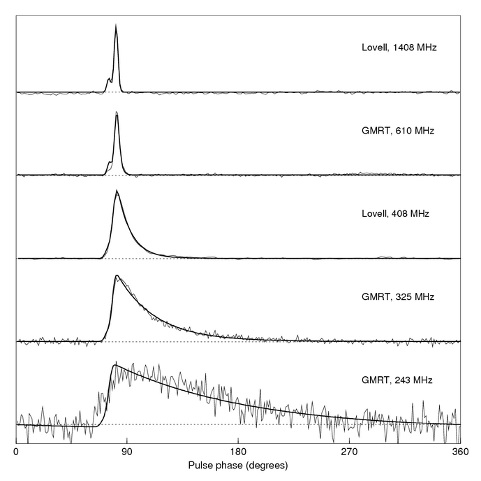
Figure 9 taken from
Pulsar Properties
at NRAO
(and taken originally from
Handbook of Pulsar Astronomy
by Lorimer and Kramer (2004).
Twisting the paths of cosmic rays
Another of our "messengers from space" are the cosmic rays: particles -- electrons, protons, and helium nuclei (aka alpha particles), for the most part -- ejected gently from ordinary stellar winds, and shot at high speed from violent events such as supernovae and relativistic jets. Almost all of these particles are electrically charged.
Q: What about neutrons?
Like any electrically charged particles, cosmic rays will be accelerated -- and therefore deflected from their original paths -- if they encounter magnetic fields. And galaxies do tend to have magnetic fields. Take a peek at our own Milky Way, in this image based on measurements of polarized radio waves from the Planck satellite.
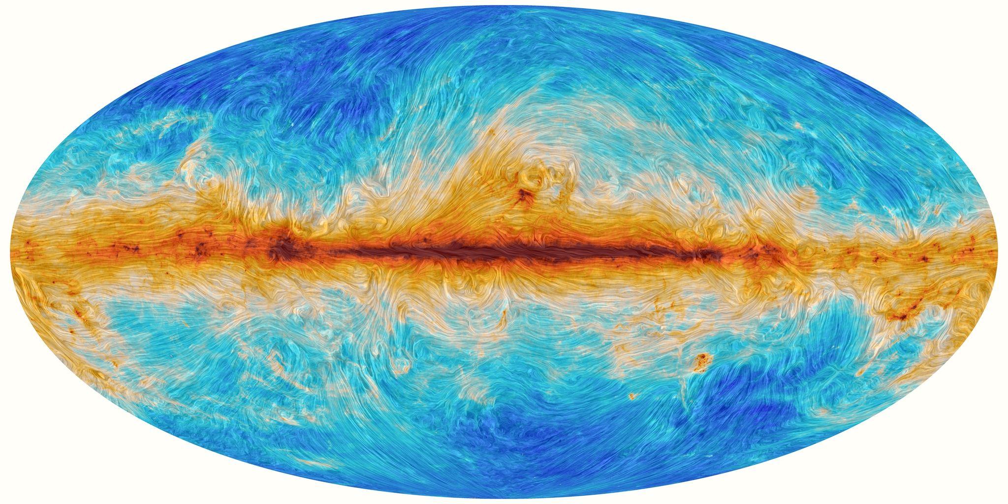
Image courtesy of
ESA and the Planck Collaboration
In some places, the magnetic field seems relatively uniform ... but if you look closely, you can find tangles and twisty passages all over the place. Near the Orion star-forming region, for example, we see this:

Image courtesy of
ESA and the Planck Collaboration
In addition to the magnetic field within each galaxy, there are magnetic fields which fill the space between them. Although these fields are weak, they exert forces over very long distances. The deflections can add up. Hackstein et al. (2016) simulate the motion of cosmic rays over distances over 1 Gpc. The figure below shows the difference between the real direction to a source and the direction from which its particles arrive. The large deflection angles out to 80 - 100 Mpc are (I believe) an artifact of their simulation method, so the real deflection should be smaller. But the rise in deflection for sources more distant than 100 Mpc is real.
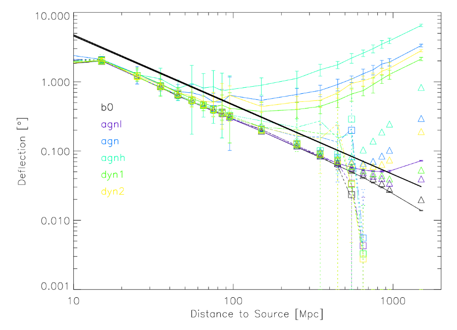
Figure 3 of
Hackstein et al., MNRAS 462, 366 (2016)
The deflection of a cosmic ray's path is decreases with the CR's energy, so we might learn more from the highest-energy cosmic rays; on the other hand, those relatively undeflected particles are much less common than the low-energy, easily-deflected ones.
Another illustration of this problem is shown by Kobzar et al., 2016. They simulate the arrival directions of cosmic rays from the nearby active galaxy Virgo A = M87, which is just 20 Mpc or so away. The figure below shows a map of the northern galactic hemisphere, in galactic coordinates: galactic latitude is +90 at the center and 0 (the equator) at the circumference, and galactic longitude runs clockwise, as shown by the labels. Virgo A's position is marked by a star, the areas in which cosmic rays from it would be detected are shown as colored shaded areas, and the directions of actual ultra-high-energy cosmic ray detections are indicated by colored dots.
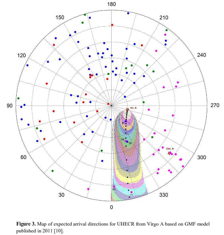
Figure 3 taken from
Kobzar et al., arXiv 1602.01683
Copyright © Michael Richmond.
This work is licensed under a Creative Commons License.