Copyright © Michael Richmond.
This work is licensed under a Creative Commons License.
Copyright © Michael Richmond.
This work is licensed under a Creative Commons License.
What is an ultraviolet photon? There are no exact definitions, so I'll adopt the following rough range:
      Energy (eV)               4     -    100

      Wavelength (Angstrom)  3000     -    120
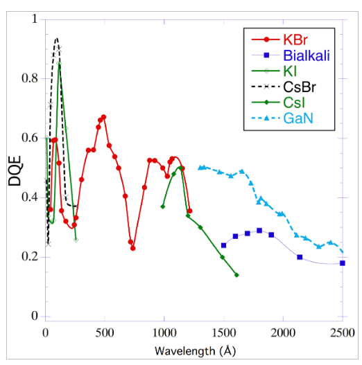
To a large extent, UV photons can be captured and measured using some of the same devices as X-ray and optical photons. Some examples with which you might be familiar are:
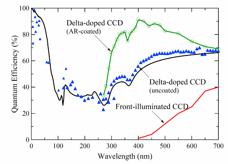
While ordinary CCD's don't reach the UV, there are CD detectors (Delta-Doped CCDs and EMCCDS) and well as CMOS detectors that are optimized for the UV. Here are just a few examples of CCDs with high QE in the UV:
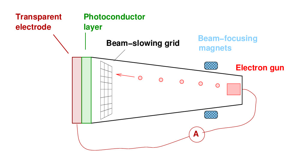
I'd like to mention one type of detector which was widely used for visible-light and UV-light imaging over the past century or so: the vidicon (and its relatives). You won't see many, or any, of these in use now, but the idea behind them is clever. And since they were used on some of the first UV satellites, such as Copernicus, this is a good time to introduce them.
The basic idea of a vidicon has two parts:
The real device is a lot more complicated than the schematic shown below, but this should give you some idea of its construction.
  Q:  Does this design remind you of any common household device?
          Or, at least, of the design of a household device
          common when your parents were growing up?
Yes, that's right -- this is sort of like a television set, run in reverse. Instead of starting with an image encoded as a pattern of currents (on, off, off, on, on, ...) and spraying electrons (under the control of magnets and electric fields) onto a phosphor screen in order to make the screen glow in a copy of the image, this device allows photons to fall onto a screen and PRODUCE an image, which is then translated into a pattern of currents by a scanning electron beam.
Devices of this sort were used for many years to produce television broadcasts: an optical image is turned into a series of electric currents, and then voltages, and then beep-beep-boops of radio waves; the radio waves reach a receiver, which turns their pattern of beep-beep-boops back into a picture on a screen.
But this sort of device can also be used for astronomy in space. A vidicon, or similar detector, could encode an optical or UV image on board a satellite, then send a radio wave with a series of beep-beep-boops back to the ground.
Some cool pictures of real vidicon tubes:
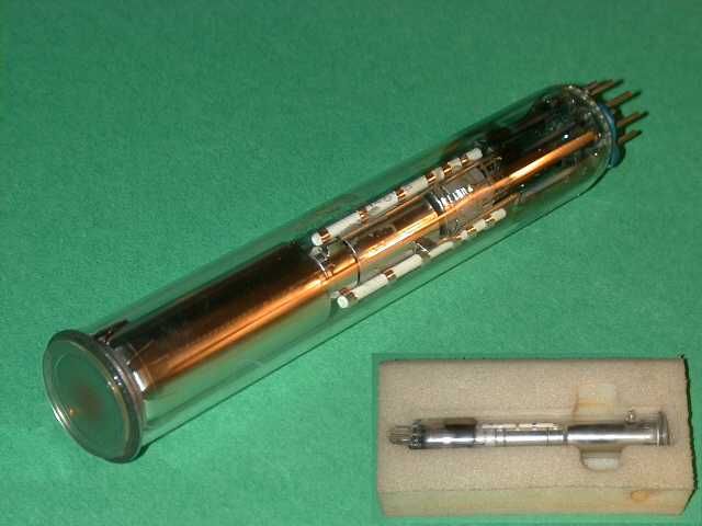
Image of RCA 6198 courtesy of
LabGuysWorld
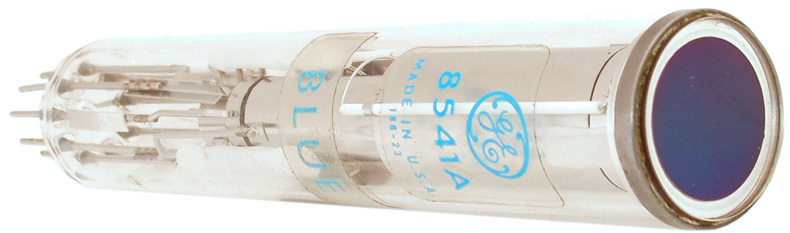
Image of GE 8541A-Blue courtesy of
SurplusSales.com,
which will sell you one for $75.

Image of Return Beam Vidicon tube, of the sort launched in Landsat 1
in 1972, courtesy of
Smithsonian Air and Space Museum
Here are some examples of images collected by vidicons.
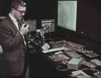
It was a different time, in some ways ...
In many cases, UV photons are similar enough to optical photons that they can be collected and focused in the same way -- with ordinary lenses and mirrors. Well, semi-ordinary, at least: the materials used to construct UV lenses can be rather exotic, such as magnesium fluoride.
But consider the telescopes placed into the Orbiting Astronomical Observatory series of satellites in the 1960s and 1970s. They are run-of-the-mill Cassegrain telescopes, with a large primary mirror and smaller secondary. Light from space bounces from the primary to the secondary, and finally heads straight back down toward the primary. In one version, the light came to a focus on a vidicon-like detector sitting in front of the primary:
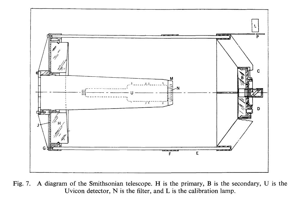
Diagram of telescope used in OAO series of satellites
taken from
Rogerson, J., Space Sciences Reviews 2, 621 (1963)
But the instrument for the OAO-3 mission, nicknamed "Copernicus", was a spectrograph, not a simple imaging camera. It was too big to fit into the shadow of the secondary mirror ... but, in the cramped confines of the small satellite (less than 3 meters long and 80 cm in diameter), there just wasn't any place to hide it behind the primary or off to the sides. So, the spectrograph's body sticks out and occults portions of the primary! Only 58 percent of the aperture is clear to incoming photons, but that's the price one pays for putting a big instrument into a small spacecraft.
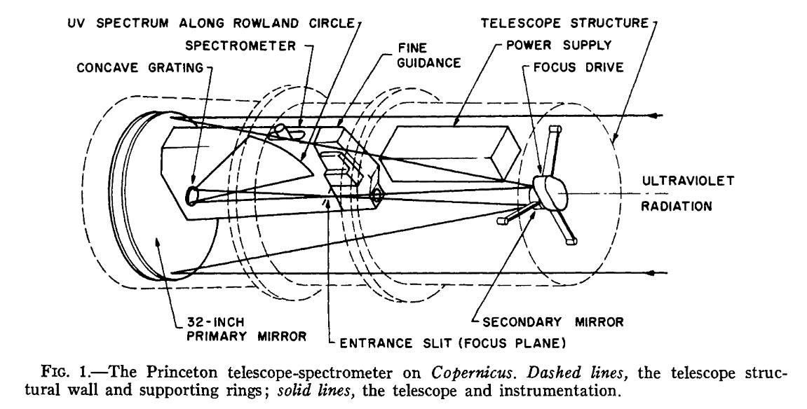
Diagram of telescope and detector aboard OAO-3, aka "Copernicus",
taken from
Rogerson et al., ApJ 181, 97 (1973)
The OAO series shows that some UV astronomy can be done with ordinary mirrors, but the range of wavelengths covered -- from about 710 to 3275 Angstroms -- did not include the most energetic ultraviolet photons. The scientists who designed the Extreme Ultraviolet Explorer (EUVE), mission, launched in 1992, wanted to roam in this hitherto undiscovered country. The satellite carried microchannel plates which could detect photons between 70 and 760 Angstroms. Those photons would reflect only poorly from ordinary mirrors, so the EUVE team had to design grazing-incidence optics reminiscent of those found in X-ray telescopes.
EUVE carried three telescopes, each with its own variety of Wolter-Schwarzschild mirrors. In the diagrams below, photons come from deep space, travelling left to right. Note that in the telescopes shown in panels b) and c), photons strike the opposing surfaces of the primary and secondary mirrors. Neat!
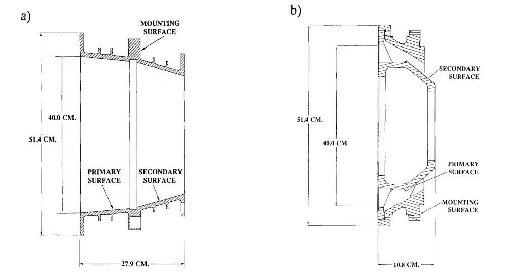
Figure 2 taken from
Bowyer et al., Highlights of Astronomy 9, 247 (1992)
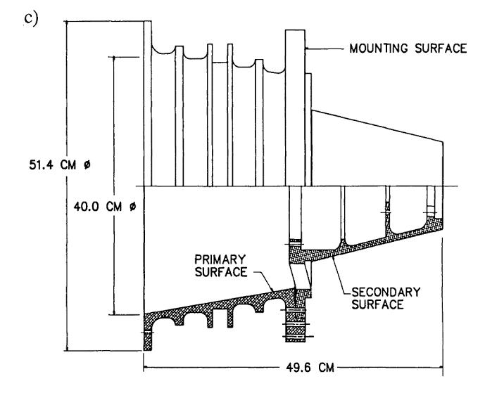
Figure 2 taken from
Bowyer et al., Highlights of Astronomy 9, 247 (1992)
Designs for modern UV telescopes and spectrographs use a lot of the same concepts. They usually have far fewer optics than optical spectrographs. For efficiency's sake, we need to limit the number of bounces. Below are diagrams for the Rowland Circle Spectrographs and Concave gratings.
Figures taken from
Vacuum Ultraviolet Spectroscopy
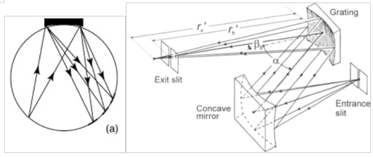
These UV optics are coated with special materials to improve their reflectivity at short wavelengths.
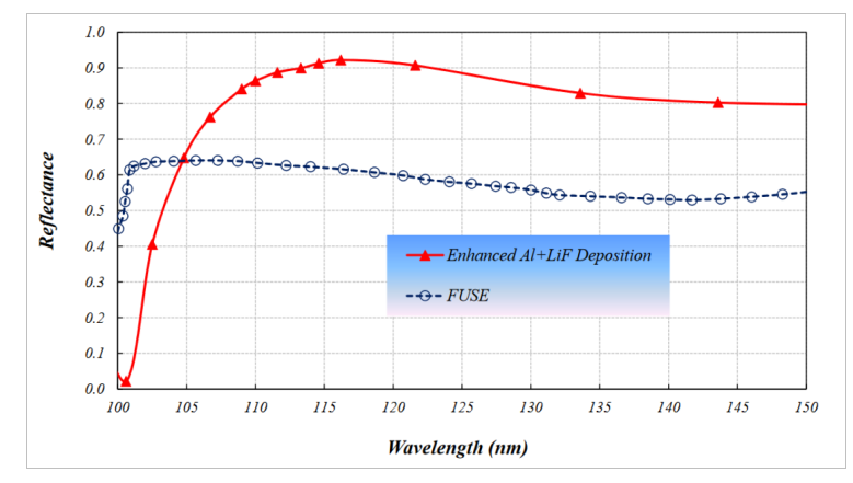
Figure 7 taken from
Tuttle, S. et al., "Ultraviolet Technology To Prepare For The Habitable Worlds Observatory", arXiv 2408.07242v1 (2024)
Most of the satellites built to study the UV have used ordinary mirrors, at the cost of being limited to the relatively low-energy end of the UV spectrum. The list below is by no means comprehensive, but merely lists a few of the instruments which do at least some work in the UV. In addition to these dedicated satellites, there have been many instruments mounted on balloons, rockets, and short duration stays in orbit.
| Mission | Active | Diameter (cm) | Wavelength (Angstroms) |
|---|---|---|---|
| OAO-3 = Copernicus | 1972 - 1981 | 80 | 710 - 3275 |
| EUVE | 1992 - 2001 | 40 (*) | 70 - 760 |
| FUSE | 1999 - 2007 | 140 | 900 - 1200 |
| XMM OM | 2000 - | 30 | 1700 - 6500 |
| Galaxy Explorer (GALEX) | 2003 - 2013 | 50 | 1344 - 2831 |
| FIMS/SPEAR | 2003 - 2004 | 71 | 900 - 1150, 1350 - 1710 |
| SWIFT UVOT | 2004 - | 30 | 1700 - 6000 |
| HST | 1990 - | 240 | FOC: 1150 - 6500 ACS: 1150 - 11000 WFC3: 2000 - 18000 COS: 900 - 3200 |
| Sprint-A = Hisaki | 2013 - 2023 | 20 | 520 - 1480 |
| ASTROSAT | 2015 - | 2 x 37 | 1300 - 5500 |
| CUTE | 2021 - | 5 | 2500 - 3300 |
| In the future ... | |||
| Aspera | 2026 - | 10 | 1030 - 1040 |
| SPRITE | 2026 - | 33 | 1020 - 1740 |
| SPARCS | 2026 - | 9 | 1530 - 1710, 2500 - 3000 |
| UVEX | 2030 - | 75 | 1390 - 1900, 2030 - 2700 |
| Habitable Worlds Observatory (HWO) | 2040s? | 600? 800? | ?? |
A good reason to study the UV: stellar absorption lines
Spectroscopy (which we will discuss in depth somewhat later) is a powerful tool for determining the chemical composition and physical conditions in stars and nebulae. In ordinary stars, we see a series of absorption lines caused by light from the hot interior of the star escaping through the cooler gases in the photosphere. As a general rule, strong lines due to neutral and ionized atoms tend to be more common in the blue portion of the optical spectrum than in the red portion.

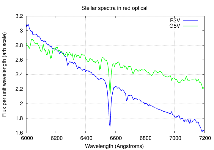
If we could detect near-UV light from stars, we'd find even more strong absorption lines with which to probe stellar atmospheres:

The near-ultraviolet region is VERY important for the study of supernovae of type Ia. These events, which occur when a white dwarf grows more massive than the Chandrasekhar limit (either via accretion from a main-sequence companion, or from merging with a second white dwarf), look rather similar when studied in optical light, but quite diverse in the ultraviolet.
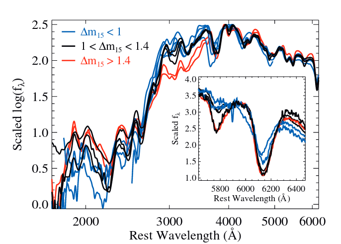
Figure 2b taken from
Foley et al., MNRAS 461, 1308 (2016)
In the figure below, spectra of two real supernovae, SNe 2011by and 2011fe, are plotted together with a model (shown in gold) which reproduces their light curves well. The upper panel shows the three spectra, while the lower panel shows the fractional difference of each real spectrum from the model. Note how the differences become much larger in the ultraviolet.
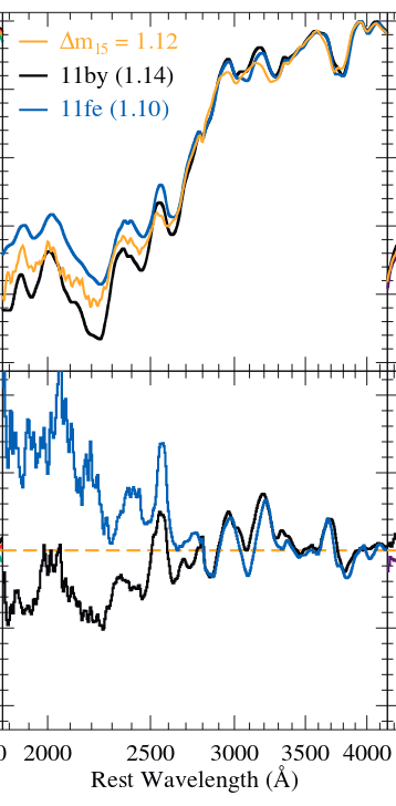
Figure 5b taken from
Foley et al., MNRAS 461, 1308 (2016)
As a final illustration of this point, the figure below shows the fractional differences between a sample of ten supernovae of type Ia, all observed near maximum light. Again, noticed how the differences between events is much easier to see if one can observe in the near-UV.
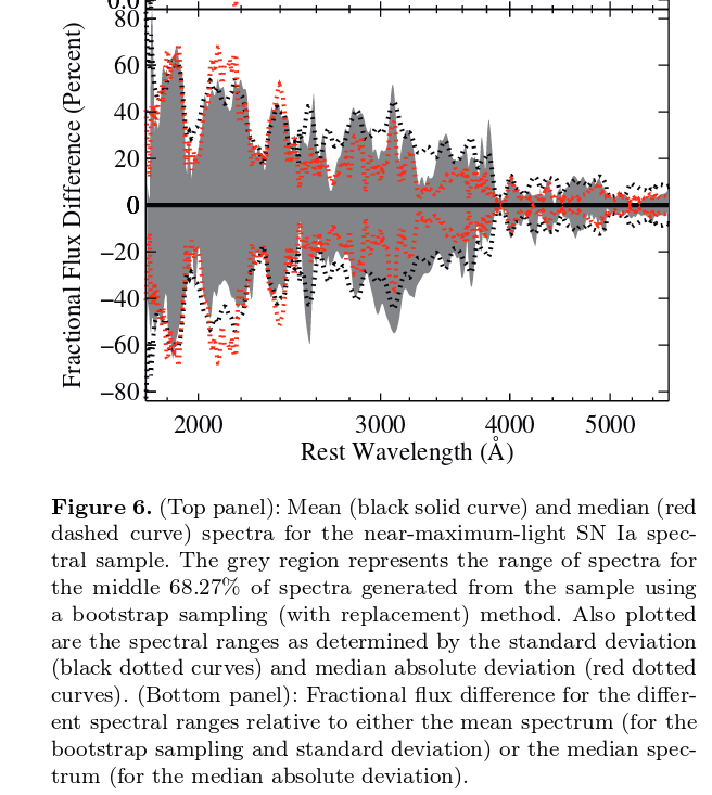
Figure 6b taken from
Foley et al., MNRAS 461, 1308 (2016)
Other good reasons to look in the UV
Lots of people want to find exoplanets -- especially exoplanets which might host life, or be hospitable to far-future human visitors. But stars which emit frequent UV-strong flares will NOT be good places for any sort of life (at least as we know it).
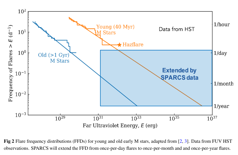
Figure 2 taken from
Shkolnik et al., arXiv 2507.03102 (2025)
Certain types of interstellar material may glow at certain wavelengths of the UV, making it possible to detect otherwise invisible clouds.
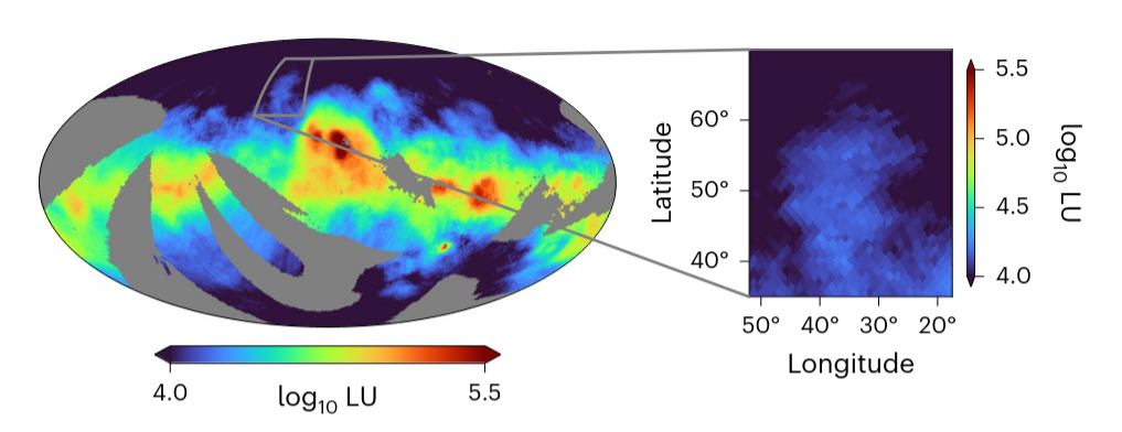
Figure 1 taken from
Burkhart et al., Nature Astronomy, 9, 1064 (2025)
Scientists interested in the circumgalactic medium expect that most of the matter will be in a diffuse, warm-to-hot phase which is best probed by its UV emission.

Figure 4 taken from
Tuttle, S. et al., "Ultraviolet Technology To Prepare For The Habitable Worlds Observatory", arXiv 2408.07242v1 (2024)
A big problem for the UV: interstellar absorption
So, there are several good reasons to try to observe stars and other celestial objects in the ultraviolet portion of the spectrum. But there's also one big problem, if one tries to look at wavelengths less than 1216 Angstroms. That problem is absorption by the ISM.
Light travelling through space needs to navigate its way past the atoms which float between the stars. As you know, if a photon encounters an atom in a low energy state, it may
Now, there are many different varieties of atom, each with its own set of energy levels, so the possibilities for absorption are legion.
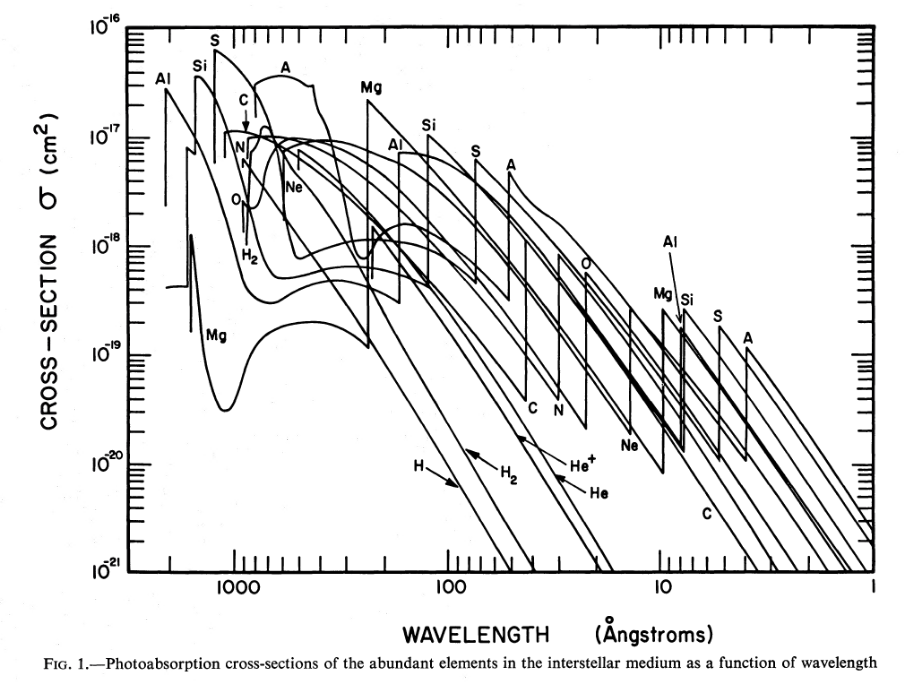
Figure 1 taken from
Cruddace et al., ApJ 187, 497 (1974)
  Q:  Do you notice a pattern to these cross sections
         as a function of energy?


  Q:  What element corresponds to the letter "A" in the graph above
         (and the one below)?
Answer to the letter "A" question
Fortunately for astronomers, most of these atoms are only infrequently found in the interstellar medium. Even though an Aluminum atom, for example, may have a large cross section for absorption, there are so few Aluminum atoms in space that their combined effect is much smaller than that of more common atoms; such as, notably, hydrogen and helium.
Cruddace et al., ApJ 187, 497 (1974) combine the cross sections of atoms of each element with their typical abundances to compute an overall effective cross section.
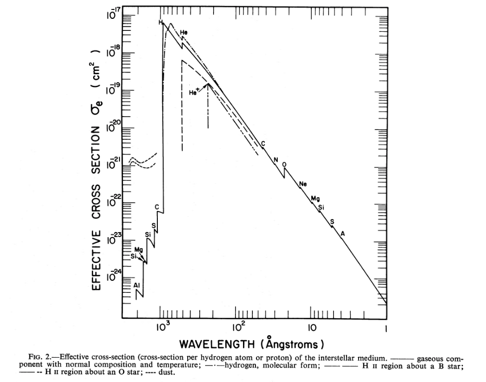
Figure 2 taken from
Cruddace et al., ApJ 187, 497 (1974)
Now, how can we use this information to figure out the effect of all these atoms on light passing through the ISM? You can read a more detailed explanation in my notes from another course, but the basic idea goes like this:
You can compute the mean free path of a photon via the equation
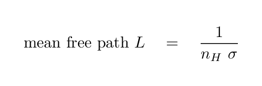
This mean free path is a useful quantity in several ways. First, value itself gives one a rough idea for the distance that a photon will travel before being absorbed or scattered (and that is the use to which we will put it today). But it can also be used to determine the optical depth of a material to radiation. If a photon travels through a slab of material which is a distance D in depth, inside which the mean free path is L, then the optical depth of the slab is
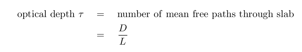
If a beam of light of initial intensity I0 passes through a slab of material with optical depth τ, then its outgoing intensity will be only

Okay, enough theory, let's do some calculation. Let's begin with a very simple, and not correct, assumption: that the number density of hydrogen is about nH = 1 atom cm-3.
  Q:  Using values of the effective cross section from
            the figure above, compute the mean free path
            for photons of wavelengths

               λ = 912 Angstroms

               λ = 100 Angstroms     (UV/X-ray boundary)

               λ =  10 Angstroms     (soft X-rays)
By the way, what is so special about 912 Angstroms?
My answer
The results should show you that the distance a hard-UV photon can travel through the ISM is ... not very far.
  Q:  How do these distances compare to

         a)  the distance to the nearest star?

         b)  the distance to the nearest star-forming region?

         c)  the distance to the center of the Milky Way?

         d)  the height of the Milky Way's disk?
Fortunately for astronomers, the ISM is not a homogeneous fog of hydrogen with exactly 1 atom per cubic centimeter everywhere. Instead, the ISM appears to consist of several components: clouds, warm gas, and hot gas. Some very very rough numbers for these phases might be
      Phase            Temp (K)       density (atoms/cm^3)     filling factor
-------------------------------------------------------------------------------
    cold clouds         100                10                      0.05

    warm gas         10,000                 0.1                    0.25

    hot gas       1,000,000                 0.001                  0.70

--------------------------------------------------------------------------------
The important feature of this "multi-phase model" of the ISM is that MOST of the volume is filled with very tenuous, very hot gas ... which is much more transparent than the material we assumed earlier.
  Q:  Suppose that if we look in one particular direction,
            we just happen to encounter only hot gas.
            For this direction, compute again the mean free path
            for photons of wavelengths

               λ = 912 Angstroms

               λ = 100 Angstroms     (UV/X-ray boundary)

               λ =  10 Angstroms     (soft X-rays)
So maybe it's not crazy to build a telescope to look for celestial sources at wavelengths below the Lyman limit, less than 912 Angstroms. In fact, that was precisely the goal of the Extreme Ultraviolet Explorer (EUVE). Over a period of six months, it scanned the sky, making an all-sky survey of sources in the range of 70 - 760 Angstroms. It detected 734 objects during this survey, and then another 500 or so objects during operations over the next few years, for a total of nearly 1200.
  Q:  How many stars are visible to the naked eye from
           a dark location on Earth?
Below is a map showing all these EUVE sources, on a Hammer-Aitoff projection in galactic coordinates.

Map of the EUVE all-sky sources courtesy of
Mikulski Archive of EUVE results
  Q:  Roughly how many extragalactic sources are there?


  Q:  Where are most of the extragalactic sources located?
Looking for a challenge? Below is a link to an ASCII datafile containing a list of all the sources detected by EUVE. The datafile contains all of the documentation I've been able to find for it.
Your challenge (should you choose to accept it):
Copyright © Michael Richmond.
This work is licensed under a Creative Commons License.