Added results of second set of linearity tests, Feb 21, 2015. MWR
On Jan 7-9, 2015, I ran several tests of HDI together with RIT students Triana Almeyda, Yashashree Jadhav, and Brandon Miller. The main goals were to check the gain of the device in single-amplifier mode, and to check the linearity.
In order to check the linearity of the camera in single-amplifier mode, we acquired a series of images of the dome-flat spot through the I-band filter. We left the lamp setting at a low level (low-intensity, about 30 percent) and changed the exposure times to cover a wide range of light levels in the images. The images can be found in the HDI archive in
c7031t0013f00.fits - c7031t0038f00.fits
Exposure times ranged from 2 seconds to 150 seconds. The tests took place after sunset, on a cloudy night, when the skies were dark. Both the dome slit and louvres were closed, so there should have been little external light inside the dome.
The light levels in the raw frames ranged from about 800 counts above bias to about 60,000 counts above bias.
The procedure was
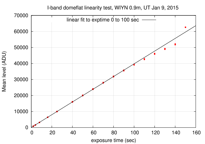
The result was 104 pairs of "exposure-and-mean" values. When one graphs the mean level versus the exposure time, one should find a linear relationship.
You can see the results in the figure below. The solid line is a fit to the measurements with exposure times between 2 and 100 seconds; or, alternatively, to measurements with light levels between 0 and 40,000 ADU.
Clearly, the linear relationship fails for high light levels. The point at which the response leaves the linear regime -- at about 40,000 ADU -- is slightly higher than the point at which the gain test, below, reveals a change in behavior.
Second linearity test: B-band, Feb 21, 2015
On Feb 21, 2015, Con Deliyannis took a set of dome flatfield images at night. He used the B-band filter, and used the low-intensity lamp at its 100% setting. Con describes his work as follows:
Ideally, we would like to identify where the CCD becomes nonlinear at better than 1% (some would say 0.5%, or even 0.1%). But this is very difficult to do, if the possibility is there that the lamps are fluctuating at >>1%. We have no direct way of knowing whether the lamps are fluctuating during the linearity tests. So I did the tests three times; perhaps if all three tests are consistent with each other, the lamps were sufficiently constant during the tests. (Would blue sky with narrow-band filter during mid-day provide a more constant source of light?? I said narrow- band hoping that multiple-second exposures won't saturate the CCD; with U, even a 1sec exposure in mid-day would saturate.)To attempt to encourage the lamps to behave, I didn't want to change from 100% low lamps, which had been on for some time. I thus chose the B filter since one can expose the longest with this filter (compared to VRI) without saturating, thus giving us a finer grid of points near saturation level, which is where any possible nonlinearity might appear. I did the following set of exposures (sec):
5, 10, 15, 20, 25, 30, 35, 40, 42, 44, 46, 48, 50 (exp# 88-98)and then repeated this set twice (exp# 99-109, 110-120).
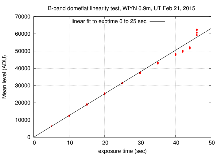
I reduced and analyzed these images in exactly the same manner as I did the Jan 08, 2015, images, above.
The results are shown below. The pattern is very similar to that of the Jan, 2015, tests: a linear relationship up to somewhere around 30,000 to 40,000 ADU, followed by a slight rolloff.
In order to check the gain of the camera in single-amplifier mode, we acquired a series of images of the dome-flat spot through the I-band filter. We modified the lamp setting and the exposure time to cover a wide range of light levels in the images. The images can be found in the HDI archive in
c7030t0013f00.fits - c7030t0057f00.fits
The light levels in the raw frames ranged from about 2000 counts above bias to about 50,000 counts above bias.
The procedure was
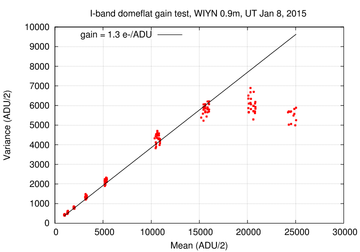
The result was 204 pairs of "mean-and-variance" values. When one graphs the variance versus the mean values, one should find a linear relationship with slope
                 1          1
   slope  =   -------  *  -----
               gain         2
where the gain has units of electrons/ADU, and the factor of 1/2 accounts for the division of all raw pixel values by 2 at the start of our analysis.
You can see the results in the figure below. The solid line corresponds to the results one would attain for a gain of 1.3 electrons per ADU, which is the value computed in Tech Note 1, in Feb, 2013 .
It is clear that
The pattern is not unlike that measured for a similar device (e2v CCD44-82) measured by Downing et al., Proc. SPIE 6276, High Energy, Optical, and Infrared Detectors for Astronomy II, 627609 (15 June 2006).