This document will describe briefly the steps one may take to turn raw HDI images into cleaned images, suitable for further analysis. This guide will consider only images with single-amplifier readout; if you want to work on four-amplifier readout images, you'll have to do some extra work.
You can find links to copies of the FITS images used as examples scattered throughout this document. There's also a list of them collected at the end.
The data used as an example herein were taken in Jan 22/23, 2014, by a team from RIT:
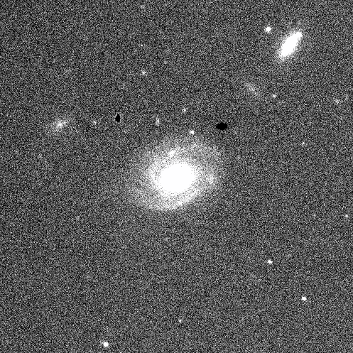
The conditions were fairly good on that night. We'll focus on images of the galaxy UGC 6719, at J2000 (RA = 11:44:47, Dec = +20:07:30). The images were taken with an R-band filter and had an exposure time of 120 seconds.
Contents:
Let's begin with the raw image.
All images from HDI are sent first to the HDI image-server computer, known as hdiserver.kpno.noao.edu. This computer saves a copy of each image into a local data archive, creates a JPEG quick-look image, the places both the JPEG and full FITS image onto a website for the user to examine.
Now, the format of this FITS image is a bit tricky. It's not a "simple" FITS image, but instead a FITS file with a single extension. What's the difference? Well, in a very simple-minded way,
               Simple FITS image              raw HDI 1-amp image
            ------------------------      ---------------------------

              FITS header                       FITS header

              image data                        FITS header

                                                image data

            ------------------------      ---------------------------
Some image display and analysis software will deal just fine with the raw HDI image; ds9, for example, will show you the entire frame (except for overscan) by default. However, some programs are confused by the "FITS-file-with-1-extension" format; you may have to specify the extension explicitly when you run a command.
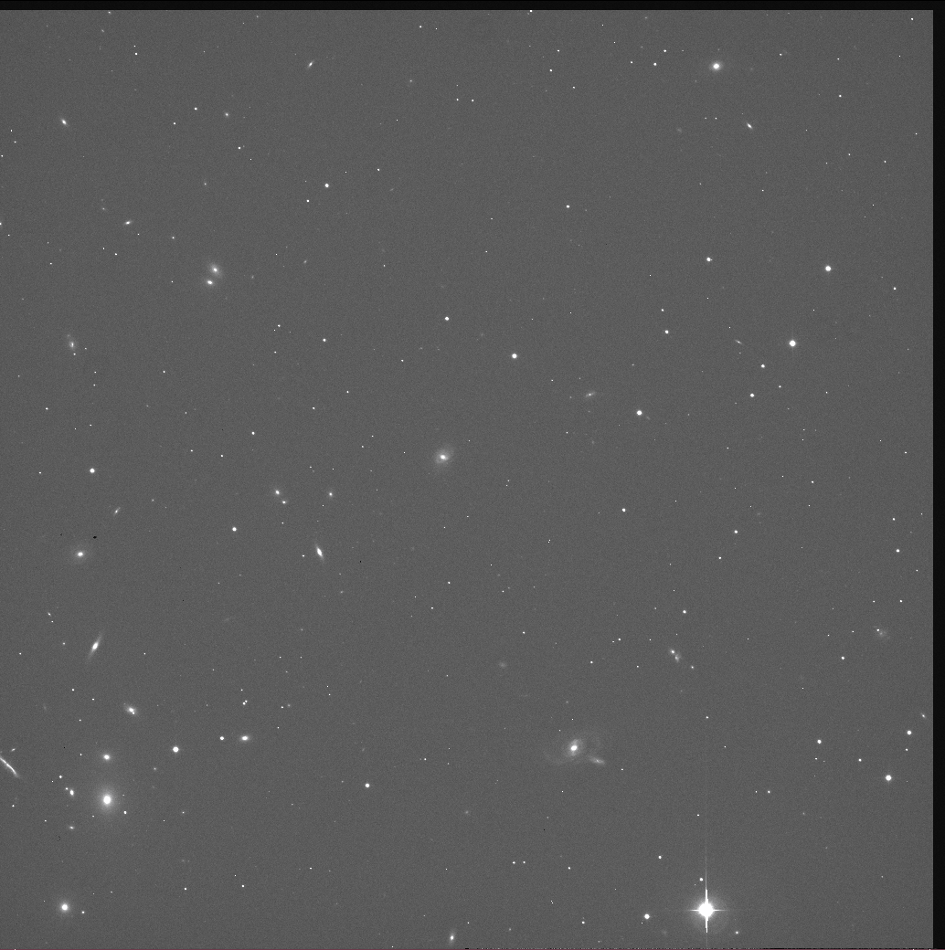
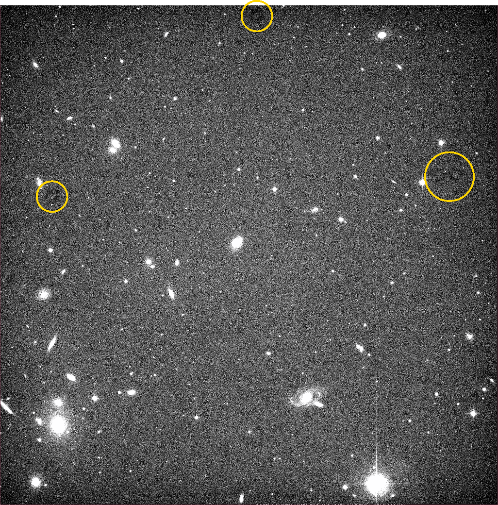
Let's look at one raw image, c6680t0131o00.fits. I'll make a copy in the "simple FITS" format for convenience:
I'll orient this and all following pictures so that they match the view you'll see if you display them in ds9: North is up and East to the right, which is flipped horizontally from the usual convention.
Now, if you look carefully at the image above, you'll see that there are narrow strips around the top edge and the right-hand side which have pixels of darker color (= fewer counts) than the rest. These regions aren't really measuring the light from the sky; instead, they record the values that the pixels in the chip ought to provide when no light strikes them. They have several names:
If you look at the FITS header, you'll see several lines which tell you exactly where these special regions occur in each image:
DATASEC = '[1:4096,1:4112]'    / Imaging area of the detector
BIASSEC = '[4097:4150,1:4150]' / Overscan (bias) area
DETSIZE = '[1:4096,1:4112]'    / Iraf total image pixels in full mosaic
DETSEC  = '[1:4096,1:4112]'    / Iraf mosaic area of the detector
So, in this HDI image, the area struck by star and sky light runs from rows 1 - 4112, and columns 1 - 4096. Remember that I've flipped the orientation of the image so that it has North up; the first row, number 1, is really at the BOTTOM of the image. Columns start at number 1 at the left-hand edge of the image, as shown.
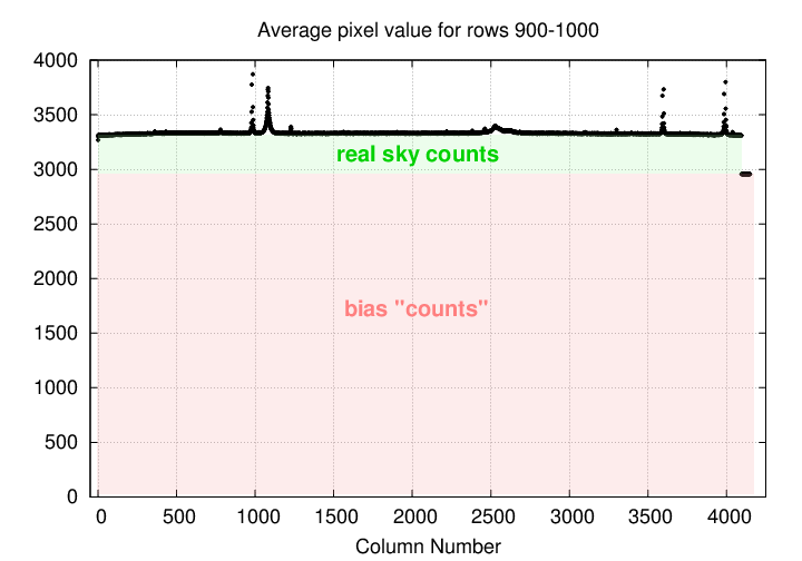
How big is the difference between the recorded number of counts in the "bias" regions compared to the "sky" regions? I measured the average pixel value in a 100-pixel wide swath running across the image from left to right (West to East). The typical pixel level is around 3300 counts, with a few sharp jumps at the locations of stars and galaxies; but the level drops below 3000 in the final 54 columns.
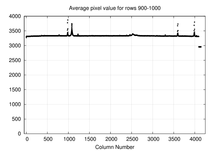
What's going on? Well, most of the counts in the real-sky area are actually just due to the bias setting of the chip. The real sky light accounts for a thin layer of counts on top of the bias.
A good first step in reducing HDI data is to remove the contribution of the bias to each image. We can use the extra overscan columns to determine this bias level: I recommend skipping the first few and last few columns to avoid edge effects. For example, you might designate columns 4100 - 4140 as overscan columns.
As you can read in HDI Tech Note 6, Properties of the overscan, and dark current , I examined a series of test images taken on Jan 22/23, 2014, and found that the pixel values in the overscan columns did not change across the length of a single image. That is, the value in rows 1, 1000, 2000, 3000, 4000, were all about the same. Therefore, we can adopt the notion that the mean overscan value is a good measure of the bias contribution to an image.
However, this overscan level DOES change over time, even during the course of a single night. See Tech Note 6 for an illustration of the size of these changes. This means that one standard technique for CCD reduction won't work very well: if we were to take a set of bias frames at the start of the night, and subtract an average bias frame from all raw images, we would NOT properly remove the bias contribution to each image.
Therefore, I suggest that one use the overscan columns in each image to calculate a mean (or median) value, and then subtract that value from all pixels in an image.
  1a.  compute mean value, M, of pixels in overscan columns 4100 - 4140

  1b.  subtract M from every pixel in image
After subtracting this mean overscan value, the overscan regions of the image should have values close to zero, with small positive and negative values. The real-sky pixels will have much larger values, often several hundred counts above zero. Since the big difference in mean level will confuse some subsequent processing steps, I suggest trimming off the overscan rows and columns at this point.
1c. create a trimmed image, keeping rows 1-4112 and cols 1-4096
The result should be an image with much lower pixel values than the original, raw version, and without those small strips of overscan pixels.
As far as I can tell at this point, no.
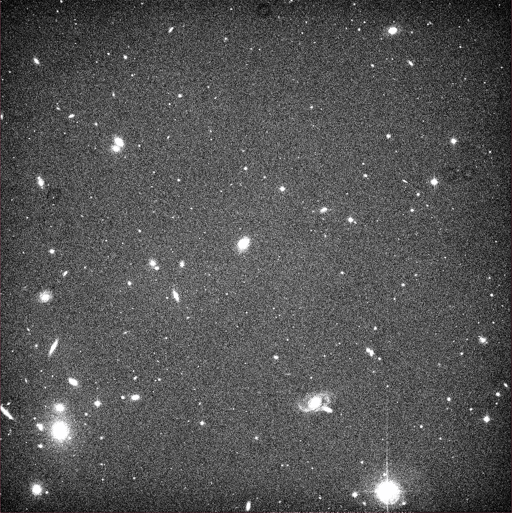
Let's look again at an image after we're subtracted the overscan value and trimmed the overscan regions. I'll choose a contrast setting that emphasizes low-level features.
Note the "donuts" visible at several locations:
There are also smaller "dark spots" in a few places; two are visible near the spiral galaxy at the middle left-hand edge of the image:
These defects are caused by material in the optical path between the sky and the camera. The big "donuts" are the shadows of dust particles on the filters or CCD window; the "dark spots" are specks of material on the CCD itself.
In order to remove their ill effects, we can use the technique called "flatfielding." Basically, we take a picture of an item which ought to be a featureless, uniform expanse of light; a perfect optical system would show an image which IS featureless and uniform. But in real life, we see the same defects in these "flatfield" images as we do in the target images: dust donuts, dark specks, sometimes slightly darker corners due to vignetting by the optics. Most of these effects are multiplicative: they block a certain fraction of the incident light. A dust donut, for example, may have pixel values only 90% = 0.90 of the surrounding pixels, meaning that only 90% of the photons from that region of the sky have reached the CCD chip. So a pixel that ought to have 10,000 counts may only show 9,000 counts.
If we divide each target image by one of these "flatfield" images, we can reverse the effects. It is necessary to normalize the flatfield image first -- that is, to scale it so that the mean pixel value is 1.0. That pixel in the middle of a dust donut will then have a value of 0.90. So, that pixel in the target image which should have a value of 10,000 counts, but only has 9,000 counts due to the shadow of the dust speck, will be divided by a value of 0.90:
       9,000 counts
      --------------   =   10,000  counts
           0.90
And thus, the pixel will be returned to its proper value after the division.
To create a proper "flatfield image", one can either take images of the sky at twilight, during a brief interval when the sky is so bright that stars are invisible, but not so bright that it saturates the detector; or one can take pictures of a white spot inside the dome, illuminated by lamps to provide the proper level of illumination. "Twilight sky flats" are probably better in a theoretical sense (from a color and uniform illimination perspective), but are certainly much more difficult to acquire.
I'll use some twilight flats in this example. Specifically, a set of six twilight R-band images, with exposure times between 5 and 10 seconds. After subtracting the overscan from each image, I computed the mean value of each image. Next, I scaled all the flatfield images so that they had the same mean value. Finally, I computed the median value for each pixel in the images to generate a master flatfield image:
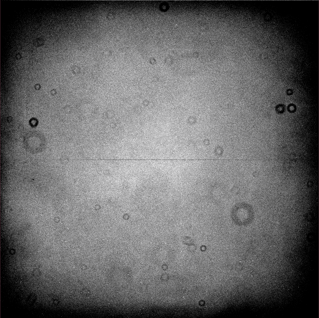
The "dust donuts" are easy to see. There are big ones due to dust specks far from the focal plane (on the filter, probably); and small ones due to dust specks closer to the focal plane (on the CCD dewar window, probably). The horizontal line through the middle of the image is a real feature of the chip: rows 2057 and 2058 are slightly lower and higher than the surrounding rows, due to a feature of the readout electronics.
We can normalize this image -- divide it by its mean value -- and then apply it to correct the target images.
2a. divide overscan-subtracted image by normalized flatfield image
The result is a "clean" CCD image without those nasty donuts.
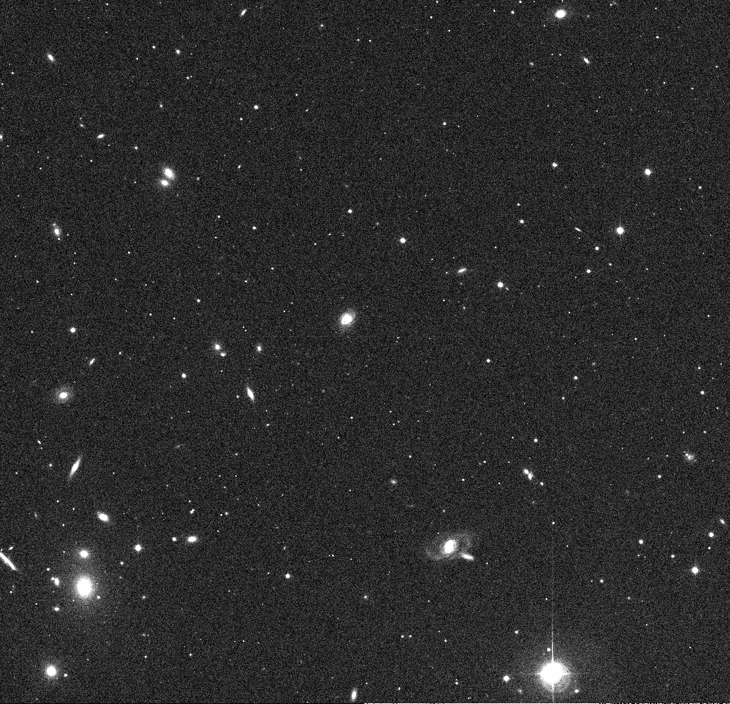
The "clean" image is much nicer than the original raw image, both cosmetically and scientifically: the pixel values in this "clean" image should be linearly proportional to the number of photons which struck each pixel during the exposure. One can use the "clean" image as the starting point for all sorts of scientific analysis: photometric or astrometric.
But there are still some annoying features which may appear in HDI images, even after the standard "cleaning" steps have been performed.
For example, the very bright star in the lower-right-hand corner of the image shows saturation, diffraction spikes, and bleed trails.

Ghosts will usually be displaced slightly from their light sources, in a direction away from the optical center of the image. This bright star is near the lower-right corner of the image, so its ghosts are displaced to the lower-right of the star, radially away from the center.
There's no simple way to remove ghosts.
In practice, it appears that the spikes running vertically (= North/South = along columns) are brighter and extend farther from the star, but this is actually due to a separate physical effect called "bleed trails."
It's not easy to make accurate models of diffraction spikes in order to remove them.
Bleed trails can travel a significant distance across the CCD, and they are difficult to remove. Most people simply mask them out and ignore the pixels they affect.
Click on each link to download the image.