On Feb 28, 2013, the new camera HDI was first used on the WIYN 0.9-m telescope. We acquired images for about one hour during the early evening, when the skies had a few wisps of thin cloud. We were unable to acquire any real darks and flats during this time, but did take images of Jupiter, M35, M44, M31 and M42.
This document describes the results of our examination of the properties of these test images.
Contents:
We had no automatic control of the shutter mechanism, so there are no precise values for any exposure times. The pictures of Jupiter probably have an exposure of around one second; all others have exposure times of around 15-20 seconds.
Exposure #	Object	Focus		Notes
---------------------------------------------
39		Jupiter	32700
40		Jupiter	32800
41		Jupiter	32600
42		Jupiter	32300
43		Jupiter	32700
44		Blank
45		M35	32800
46		M35	33000
47		M35	33200
48		M35	32900		tightened screws
49		M35	32900
50		M35	32600
51		M35	33200
52		M44	32900
53		M44	32600
54		M44	33200
55		M31	32900
56		M31	32600
57		M31	33200
58		M42	33200
59		M42	32900
60		M42	32600

--------------------------------------------------
The raw HDI images have an overscan region consisting of 48 columns along the outer edge of each quadrant of the image (all images were read through 4 amplifiers). We computed a mean value and standard deviation based on all the pixels in this overscan region.
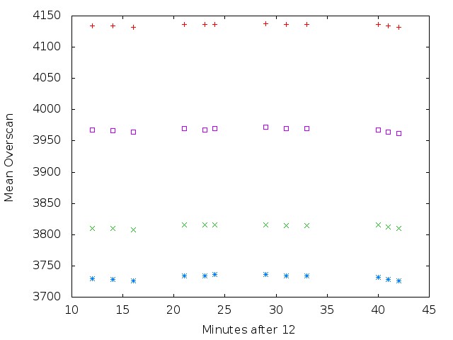
The graph below shows the mean value in each of the 4 overscan regions for each exposure. The symbols correspond to
There was little change in the mean values over the course of the roughly half hour during which we acquired data.
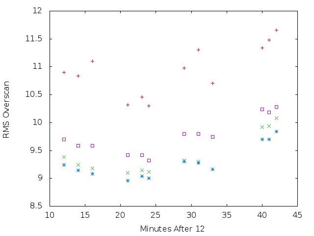
We also computed the standard deviation from the mean within each overscan region. As the next section shows , this value is not really measuring the random scatter around a fixed mean value. Nonetheless, we show the results here for completeness.
Overscan values as a function of row position
We examined the overscan regions in a second manner. The overscan pixels define a region 48 columns wide by 2056 rows tall, making a long, skinny strip running north-south. We computed the average value of the pixels in each row of the overscan region, then looked for variations as a function of row. We found a very consistent pattern: the values decline steeply at first, then gradually, with a total change of about 15 counts from top to bottom.
Below is a graph showing this average value (on the y-axis) as a function of row number (on the x-axis) for image 49 (in-focus image of M35), quadrant 1 = North-East amplifier:
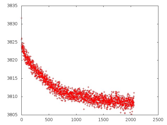
The other amplifiers produced a very similar pattern for this image; and, in general, all 4 amplifiers produced a similar pattern in all the cases we examined.
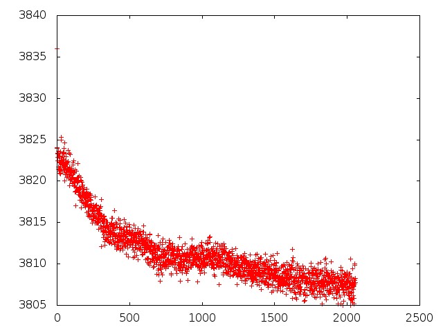
Below is the same graph for quadrant 1 of image 55:

Below is the same graph for quadrant 1 of image 60:
We find that in order to fit a smooth polynomial function to the mean value as a function of row, one needs to employ a sixth-order polynomial. The scatter around the fitted polynomial grew smaller from the start of our test images to the end of the test images; this scatter was perhaps 4-5 counts peak-to-peak at worst, decreasing to 1-2 counts peak-to-peak at best.
The gain of a CCD is the conversion factor between
electrons in the chip and counts (or Data Numbers (DN), or
Analog-to-Digital Units (ADU)) in an image.
The proper way to measure this quantity is to take a
series of flatfield images with different mean values,
as described in this lecture.
We were unable to acquire such a dataset with HDI.
However, at one point, we took a short exposure while
the telescope was pointed at a random portion of the inside
of the dome (not the uniform "flat-field spot" which
usually serves the purpose).
This exposure, number 29 in the set of images
acquired on Feb 28,
has a mean level of roughly 14,000 counts.
If we assume that the scatter in the value from
pixel-to-pixel is Poissonian, due to random fluctuations in
the number of photons striking the detector,
we can use the statistics of counts in the image
to estimate the gain.
A very cursory calculation yields a value of
gain = 1.2 +/- 0.2 electrons per count.
The designers of HDI told us that the value
should be close to 1, so this is at least consistent
with expectations.
A very rough estimate of the gain