CCD Gain

When discussing the physics of Charge-Coupled Devices (CCDs), I described how photons knocked electrons free, and how one could move electrons via electrodes placed on the silicon surface. On the other hand, when discussing the properties of CCD images, I used the word "counts" to describe the value of each pixel. What's the relationship between electrons and pixel values?

The answer is ... it depends on the chip and the software used to read it out. The steps involved in reading the value of a pixel are something like this:

Electrons transferred to "amplifier"; really a capacitor. Units are coulombs.
The voltage induced by this charge is measured. Units are volts.
An Analog-To-Digital (A/D) unit converts the voltage into some other voltage, which may have only one of several discrete levels. Units are still volts.
The voltage is converted into a number which is passed from the hardware to the computer software as the pixel's value. Units are counts, also called "Data Numbers" (DN) or "Analog-to-Digital Units" (ADUs).

In both steps 3 and 4, one can scale the result by any arbitrary factor and the relative pixel values will remain the same. Some software allows the user to modify the scaling factor dynamically; others have a fixed setting.

The end result is that there is some "fudge factor" which relates the initial number of electrons in a pixel to the final number of counts reported by camera software. The ratio of these two numbers is the gain of the camera:


                      # of electrons per pixel
          gain   =  --------------------------
                      # of counts per pixel

How should one choose the gain factor? There are several criteria.

Full-well depth vs. largest pixel value: Each CCD is designed to hold only so many electrons within a pixel before they start to leak outwards to other pixels. This maximum size of a charge packet on the chip is called the full well depth. There is also a "maximum possible number" in the Analog-to-Digital converter. Most CCDs use 14-bit, 15-bit, or 16-bit A/D units: the corresponding maximum pixel values are 2^14 = 16384, 2^15 = 32768, and 2^16 = 65536.
It is logical to arrange the gain so that very roughly, the number of electrons in the full-well depth corresponds to the maximum pixel value.
Readout noise vs. smallest pixel value: One can look at things the other way around: what are the SMALLEST values that make sense? Amplifiers on CCDs have a certain level of random noise: each time one reads the charge in a packet, one gets a slightly different value. A typical readout noise is 5 or 10 electrons RMS (meaning that the standard deviation of a bunch of measurements of the same packet would be about 5 or 10 electrons). Therefore, if two pixels have values which differ by only 3 electrons, it's not easy to tell the difference between them.
The smallest difference one can represent in an integer image is 1 count. To some extent, it makes sense to arrange the gain so that 1 count corresponds to some moderate fraction of the readout noise. Any finer measurement of the pixel values would yield differences which would be essentially random.

The CCD camera we attach to the 12-inch telescope, our "old" CCD camera, is model ST-8E from the Santa Barbara Instruments Group (SBIG for short).

Exercise:

Find the home page of the SBIG company.
Look up the gain of our ST-8E camera. What is it?

Measuring the gain factor -- a simple (and inaccurate) method

It is possible for you to check the value provided by a manufacturer. The basic idea is that if you look at a constant source of a LOT of photons (either a star, the twilight sky or a bright piece of cardboard), then the number of photons which strike the CCD in a series of exposures won't be exactly the same. Instead, the number of photons will have some scatter around an average value. The standard deviation of the number of photons should be


        stdev (photons)  =  sqrt(number of photons)

Why? Because photons coming from a star are a good example of a random Poisson process. You can look up more about the statistics of Poisson processes in the library, or in a statistics text book.

So, if you were to take a series of pictures of a bright light source which averaged 16,000 electrons in each pixel, and calculate the mean and standard deviation of the number of ELECTRONS, you'd find


        mean  (electrons)  =   16,000   per pixel
        stdev (electrons)  =      126   per pixel

However, when you measure pixel values from an image, you are actually measuring counts, not electrons. If the gain were exactly 1 electron per count then


                               mean (electrons)        16,000
        mean (counts)      =   ---------------    =  ------------  =  16,000
                               electrons/count            1
                             
                               stdev (electrons)        126
        stdev (counts)     =   -----------------  =  ------------  =     126
                               electrons/count           1

Note that


        stdev (counts)     =   sqrt( mean counts )

But suppose that the gain was set to 4 electrons per count. Then the conversion from electrons to counts changes things:


                               mean (electrons)        16,000
        mean (counts)      =   ---------------    =  ------------  =   4,000
                               electrons/count            4
                             
                               stdev (electrons)        126
        stdev (counts)     =   -----------------  =  ------------  =      32
                               electrons/count           4

Now, because of the gain factor, the standard deviation of the number of counts per pixel is NOT the same as the sqrt of the number of counts:


        stdev (counts)     =    32    

        sqrt (mean counts) =    sqrt(4,000)  =  64

In fact, you can see that we can figure out the gain by looking at the statistics of the counts:


                                       2
                [  sqrt(mean counts)  ]
        gain  = [ -----------------   ]
                [   stdev (counts)    ]

However, this simple method only works if there are no sources of noise in the CCD, so that the number of electrons is given exactly by photon statistics. Any real CCD has several sources of noise, so this technique won't yield precise results (though it ought to get in the ballpark).

Exercise:
Go to your home directory.
Copy a set of images I took several years ago with our ST-8E camera, using the following commands.
      cp $dd/gain/*.fit .
There are two sets of images: those with names including an "_a" are read directly from the CCD, unbinned, while those with names including "_b" are binned 3x3. For now, consider only the unbinned images, such as dark1_a-001.fit and light4_a-002.fit.

There are five dark frames for each exposure time: 1, 2, 4 and 8 seconds. Create a median dark frame for each exposure time; call them dark1.fit, dark2.fit, dark4.fit, dark8.fit.
Okay, let's try this simple method to measure the gain. Pick one of the 4-second exposures with names like light4_a-00?.fit. These are out-of-focus images of a piece of white posterboard attached to the inside of the dome.
Make a copy of your image.
Subtract the median 4-second dark frame from the copy
Define a box around 40 pixels on a side somewhere in a relatively smooth area of the image. Pick some region of the image far from any dust rings -- suppose it's at row=100, col=53. You can define a box centered here like so:
               box 1 cr=100 cc=53 nr=40 nc=40
        
Calculate the mean and standard deviation (aka rms) in this box
Use the equation above to get a very rough idea of the gain

What value do you get? Does it agree with the manufacturer's claim? Compare your results to those of your neighbors.

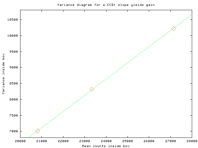
Measuring the gain -- a better technique

A better way to measure the gain is to use pairs of flatfield exposures at different signal levels. The idea is to measure the signal and variance of counts in several pairs of images, at different light levels, and then make a plot of variance vs. signal. In brief, here's how to do it.

Exercise:
pick one pair of 1-second flats (the ones called light1_a-00?.fit), one pair of 2-second flats, and one pair of 4-second flats.
for each pair, do the following:
make a copy of each image of the pair; call them copyA.fit and copyB.fit
subtract the appropriate median dark frame from each copy
add the two copies together, dividing by two, to make a summed image with the same average level as each individual image.
             add copyA.fit copyB.fit div=2 outfile=sum.fit
     
subtract the two copies to make a difference image:
             sub copyA.fit copyB.fit outfile=diff.fit
     
display the summed image. Define a box which avoids any really bad pixels or image defects. Try to make a box between 40 and 100 pixels on a side.
calculate the mean value of pixels inside this box in the summed image. Call this Mean level
calculate the standard deviation (rms) inside this box in the difference image; then determine the variance within an individual image like so:
                 variance  =  (rms)*(rms) / 2.0
       
Call this Variance
when you have done this for all three exposure times (1, 2, and 4 seconds), go to the front of the room and write down your values for "Mean Level" and "Variance" on the board.
return to your seat and make a graph on the paper provided: place "Mean Level" on the X-axis and "Variance" on the Y-axis.
calculate the slope of this graph
the slope of this graph is the reciprocal of the gain of the camera. So the gain of the camera, in electrons per count, is given by
        gain = 1/slope
     

Your graph should look something like the example below, although the numbers may be very different.

Calculate the gain by this method. How does it compare to your previous value, by the simple-but-approximate technique? How does it compare to the manufacturer's value?

Graph of measurements from Oct 2003 tests

For more details on measuring the gain of a CCD camera, see

Measuring the Gain of a CCD Camera, a tech note from Axiom Research.
Direct CCD Gain, Read Noise, and Linearity a lab exercise in the course on Observational Astronomy at Rutgers. This lab provides yet another way to calculate the gain of a CCD camera, one which doesn't require making any graphs.
Evaluating CCDs in ordinary DSLR cameras from Chritian Buil's website.