I've examined the ensemble photometry outputs of quad 1 of 20191120. This note shows some statistical properties of the objects contained in the ensemble output. It also discusses briefly how one can find moving objects by analyzing the ensemble-level output of the pipeline.
The weather was fair that night, and the observations lasted about 41 minutes. All 84 chips produced good results.
As the FITS headers of one of these images states, this data was taken in 2Hz mode:
OBJECT  = 'J0337+1648_dith1'   / object name
EXPTIME =            59.988480 / [s] total exposure time
TELAPSE =            60.500020 / [s] elapsed time
EXPTIME1=             0.499904 / [s] exposure time per frame
TFRAME  =             0.500000 / [s] frame interval in seconds
DATA-FPS=             2.000000 / [Hz] frame per second
DATA-TYP= 'OBJECT'             / data type (OBJECT,FLAT,DARK)
OBS-MOD = 'Imaging'            / observation mode
FILTER  = 'BLANK'              / filter name
PROJECT = 'Earth Shadow 2Hz Survey' / project name
OBSERVER= 'Noriaki Arima'      / observer name
PIPELINE= 'wcs,stack,raw'      / reduction pipeline templete
Now, the pipeline produces output of two kinds:
This note examines some properties of objects in the ensemble output data.
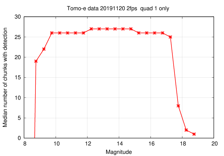
During this night, the camera pointed at a few locations and acquired multiple images in each chip at each location. Each set of 120 images were packaged together into a "chunk", and the objects in that chunk were collected into an ensemble. We expect bright objects should appear in all chunks at one particular location -- since they should appear in all images -- while very faint objects might not appear in some chunks.
The graph below shows the median number of chunks in which objects appeared, as a function of their magnitudes. And, indeed, we see the expected pattern: objects brighter than mag 17 are detected in many chunks, while very faint objects are detected in only a few.
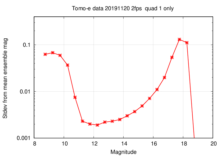
Next, let's examine the measurements of brightness of the objects. Each chunk of 120 images yields a single, average magnitude for an object, reported in the ensemble output. If a non-variable object is detected in multiple chunks, we expect that its magnitude ought to be the same in each one. For objects detected in multiple chunks, I computed the mean and standard deviation of all the reported magnitudes. The graph below shows the results.
At the bright end, magnitude measurements suffer from saturation at V < 10; and at the faint end, the uncertainty grows quickly fainter than V = 16.5 or so.
You can see the value of the uncertainty for stars between these limits more clearly in the graph below, which uses a logarithmic scale on the y-axis.
Most objects do not move appreciably during the course of a single night. Therefore, our repeated measurements of their positions should yield the same value. The scatter around the mean position is an indication of the precision of our measurements of position. The graph below shows that scatter around the mean position of objects measured in multiple chunks.
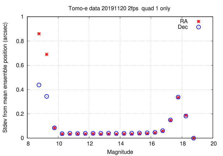
Just as the photometric values are bad for stars brighter than V = 10, the astrometric positions are also poor for these saturated stars. The same is true for the very faint stars: the uncertainty in both the magnitude and position increase after V = 16.5 or so.
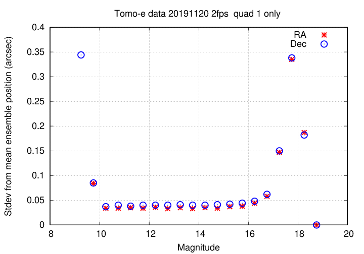
The same information is shown in the graph below, but I have zoomed in on the y-axis in order to show the precision for stars of intermediate brightness. For these "good" stars, the positions repeat to within about 0.05 arcseconds.
One can search for moving objects in a large dataset in many ways. I chose a method which is probably not a great one, but which was easy to do with the ensemble output. Remember, the ensemble method produces just one position for each chunk of 120 images.
The method was as follows:
           RA  =   a  +  b*JD

          Dec  =   c  +  d*JD
Remember, the timespan covered by these measurements is at most 41 minutes. Therefore, this technique can only detect objects with considerable speeds, of at least several arcseconds per hour.
In the quadrant 1 dataset, there were a total of 59 sources identified as having "significant" motion. The graph below shows the motions of each one.
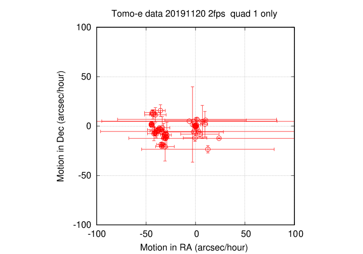
There are two main groups: one centered around an RA motion of -35 arcseconds per hour, and a second group centered around RA motion of 0 arcseconds per hour. In the following text file, the two groups are separated by a set of blank lines:
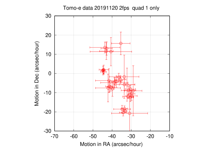
The first group has motions consistent with those of main-belt asteroids:
In order to identify objects, one can use the
For example, entering into this webpage the time of the observations (Date = 2019 11 20.61 UT), the observatory code for Kiso (381), and the position for the first item in the list (source ID 8238 RA = 03 29 59.0 Dec = 19 26 59.0), then clicking on "Produce list", yields the identification
 The following objects, brighter than V = 19.0, were found in the 5.0-arcminute region around R.A. = 03 29 59.0, Decl. = +19 26 59.0 (J2000.0) on 2019 11 20.61 UT:

 Object designation         R.A.      Decl.     V       Offsets     Motion/hr   Orbit  Further observations?
                           h  m  s     °  '  "        R.A.   Decl.  R.A.  Decl.        Comment (Elong/Decl/V at date 1)

  (4024) Ronan           03 29 59.3 +19 26 59  15.3   0.1E   0.0N    44-     1+   28o  None needed at this time.
Note that the motion computed from the Tomo-e measurements is a good match to the prediction in this case:
              measured                        prediction
            (arcsec/hour)                   (arcsec/hour)
------------------------------------------------------------------

RA           -44.70  +/-  1.20                  -44

Dec            1.55  +/-  2.28                    1

------------------------------------------------------------------
The second group of moving sources is centered near the origin:
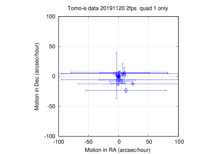
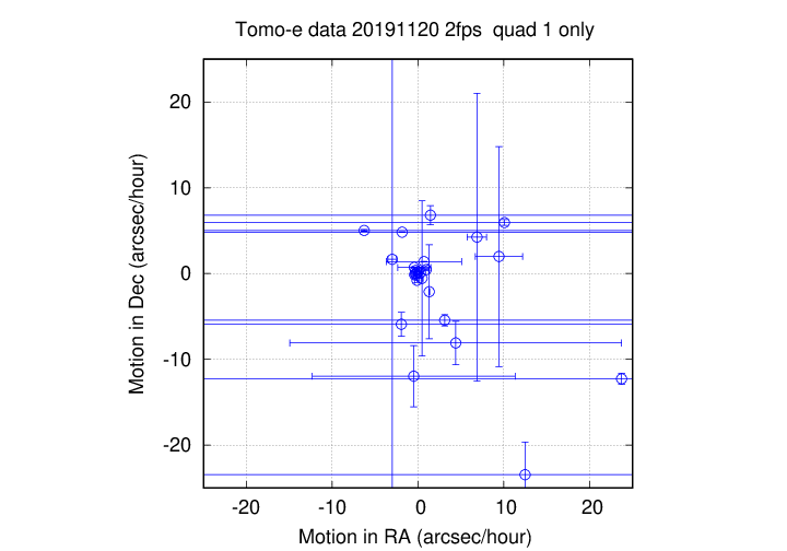
In most cases, I believe that these motion are NOT real, but simply chance combinations of a small number of positions which are really random noise around a fixed position, but happen to produce an apparently linear trend. Note how the uncertainties in most of these objects are very large.
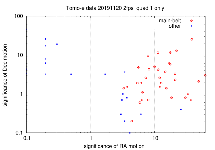
I'm not sure if the graph below is useful, but in trying to figure out which motions were real, and which spurious, I tried plotting the significance (measured motion / uncertainty in motion) in Dec vs. the significance in RA. Can one use this diagram to distinguish real from spurious motions?