Executive summary:
Table of contents
The data consist of catalogs made from Subaru Hyper-Suprime-Cam images taken on three nights:
On each night, the telescope took a series of images of different fields; usually, 3 images per field, separated by about 1 hour; however, on MJD 57166, the gap between first and second images during the night was longer, up to 5 hours.
The images were analyzed by the HSC pipeline into catalogs of detected objects. I examined the objects in these catalogs,
Although there were many different choices for the measurement of flux for each object, I chose the following:
I converted each object's flux into an instrumental magnitude using the formula
    corrected flux  =   flux_cron * flux_cron_apcorr

                                         (  corrected_flux   )
    instrumental mag  =  0 - 2.5*log10 * ( ----------------- )
                                         (  6.3095734448E10  )
The constant value 6.3095734448E10 was read from the headers of the FITS tables. I verified later that this procedure yielded g-band magnitudes which agreed with SDSS photometry of stars in the same fields very well, with a small offset of about 0.15 mag.
Each field is very large -- about 1.2 degrees wide. For convenience, each field is broken in patches which are small enough to display and process easily. Each patch is about 4000 pixels on a side, and thus (4000 pix * 0.16875 arcsec/pix) = 675 arcsec = 11 arcmin on a side.
Patch (i,j) has location as follows:
So, patch 0,0 is at South-East corner, patch 0,1 is just above it, patch 0,2 is just above that, etc. Patch 10,0 is at South-West corner, patch 10,1 is just above it, and patch 10,10 is at North-West corner.
I worked on only 4 of the fields observed on these nights: the fields with the largest number of g-band images. Each had 9 images spread over the 3 nights. The (RA, Dec) field centers listed below are only approximate.
| field | RA | Dec |
| BOO2C | 210.019230 | 14.507637 |
| MD07_I | 213.743825 | 52.815649 |
| SDSS1632 | 248.047719 | 35.050685 |
| SMSN1524 | 231.120651 | 48.112201 |
The HSC pipeline brought all the objects in all the images to a very nearly equivalent flux level. That's good -- it makes comparing the measurement between images easy.
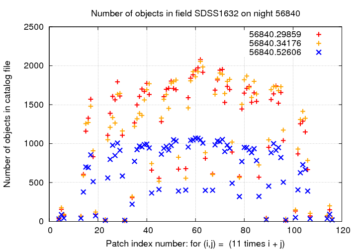
However, there is a drawback to this approach: it makes it difficult to recognize that some images may have had significantly higher noise properties (such as sky background or large PSF) than others. I discovered that some images MUST have had some sort of problem by counting the number of objects detected in each one. For example, in the SMSN1524 field, on night MJD 56840, we see:
The third image on this night, taken at MJD 56840.52606, has only about half as many detected objects as the other two images on the same night.
The images with significantly fewer detected objects are
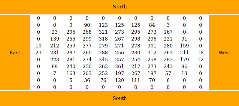
If one plots the number of objects detected within each patch for a particular field, one will see an obvious pattern: fewer objects in the outer regions of the field of view, and more objects near the center. (The table below shows the number of objects included in the ensemble processing, which is described later, but it illustrates the point).
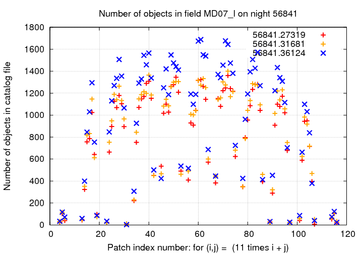
If we create a simple index for simplicity in plotting the results,
index (i, j) = 11*i + j
we can see the pattern of dips-and-rises as the index moves along columns and then to the next row. Below is a graph showing the number of objects detected in each patch for the field MD07_I. Note that the number of objects detected in the central patch -- indicated by the peak value at each rise -- of each column is about the same
On the other hand, a similar diagram for the field BOO2C shows a prominent feature: a giant spike in the patch (5,5):
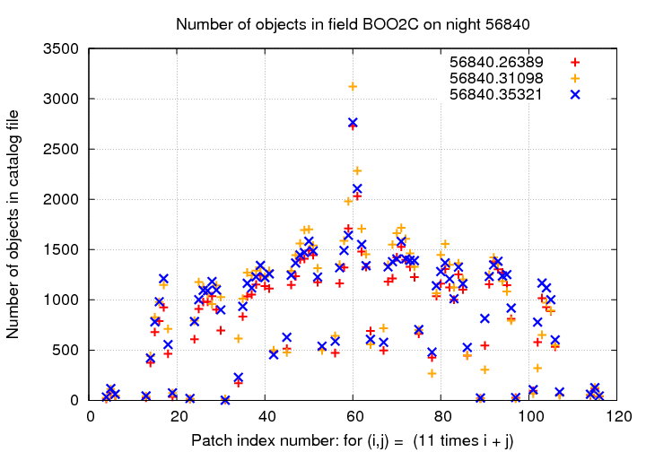
There are nearly twice as many objects in this patch as in any other patch in the field.
The reason is simple: there is a satellite galaxy of the Milky Way, known as the Bootes (or Bootes I) dwarf galaxy. It is centered almost exactly on patch (5,5) at RA = 14:00:06, Dec = +14:30:00. The distance to this satellite is about 60 kpc, so the distance modulus is about (m - M) - 18.9.
Any RR Lyr stars in this galaxy would have an apparent g-band magnitude of about 19.6. As we will see, a number of such RR Lyr are easily detected in the HSC data.
The fact that we see no other similar spike in number of detected objects in other patches or other fields suggests that there are no other MW satellites in this dataset.
The first step in my analysis was to create an ensemble for each patch's measurements. The basic idea of ensemble analysis is to identify and remove small image-to-image offsets in photometric zeropoint, to improve the precision of measurements. You can find it explained in more depth at
To discard the large number of false and "junk" detections, I placed a requirement that
in order to be included in the subsequent analysis.
The analysis procedure
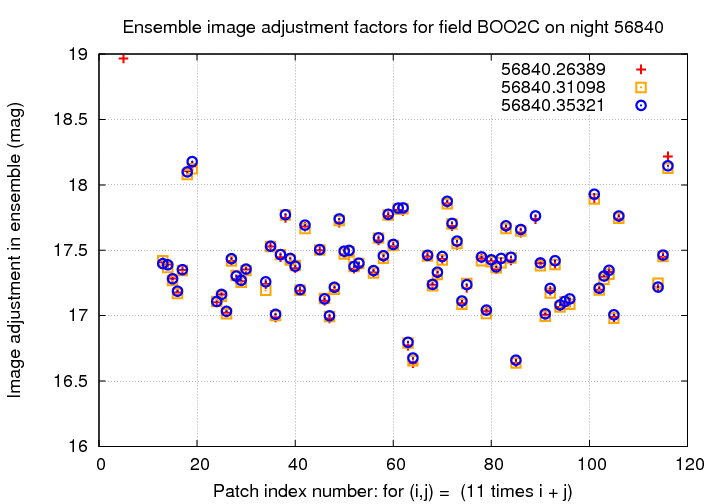
The analysis revealed that the relative photometric calibration of images for a given patch is very good. The shifts needed to bring the stars in one image into agreement with the stars in a subsequent image were very small; a typical graph is shown below. Note how small the differences in zeropoint between the three images of this patch are (in other words, how closely the three symbols for each patch overlap):
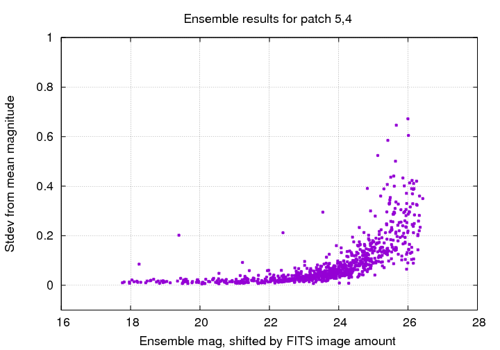
It also provides an estimate for the expected scatter in photometric measurements as a function of magnitude. The results for a typical patch look like this:
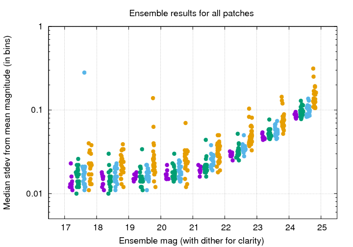
A summary of the sigma-vs-mag for all the patches in the BOO2C field shows that the scatter
The ensemble analysis produces magnitudes which are purely relative, starting at "zero" for the brightest objects in a region. In order to bring the ensemble results approximately onto the standard SDSS magnitude system, I used the bright, unsaturated stars to define an offset between the input magnitudes (based on the FLUXMAG0 value in the FITS header) and the ensemble magnitudes; then, I added that offset to all ensemble magnitudes.
To check that this offset was approximately correct, I compared the magnitudes of bright stars to the values for those stars in the SDSS DR12. There were only 2-10 stars per patch, typically, but the results show a good consistency:

There was a small offset of about 0.15 mag between my values and the real DR12 magnitudes. I did not correct for this offset in the subsequent analysis.
There were no systematic, significant variations in flux calibration from one region of the camera to another. In other words, the photometric calibration appeared to be uniform across the entire field.
In order to find RR Lyr stars, I looked at the ensemble analysis output and selected as "candidates" all objects with
Here, Nsig is the ratio of a star's measured scatter to the scatter of other stars of similar brightness. In the diagram below, you can see several candidates at the bright end. The object at avg mag = 19.5 has a scatter of about 0.20 mag, while other stars of similar brightness have a scatter of only 0.015; thus, that candidate has Nsig = 13.
I plotted the light curves of all candidates and inspected them visually. Below is a sample graph, showing all the candidates in patch (5,4) of the BOO2C field. I have shifted the measurements for the Season 2 in time so that they are appear after an apparent gap of 2 days, rather than the actual 325 days.
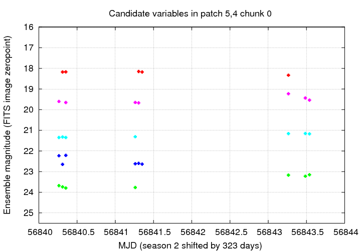
The bright candidate appears here in magenta symbols at mag = 19.5 or so. This is (probably) not an RR Lyr, but a variable of some other type.
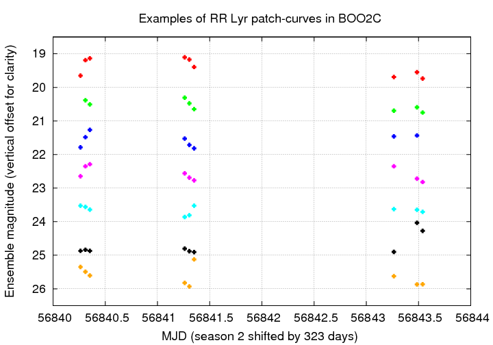
The pattern made by RR Lyr in these diagrams is rather distinctive. Below is a set of real RR Lyr curves from the dataset; each star has been shifted vertically in magnitude for clarity. The top 4 examples are RR Lyr type c, while the bottom 3 are RR Lyr type ab.
How well did this method work? We can use the Siegel (2006) set of 15 RR Lyr in the BOO2C field as a check. My visual scan (performed several times in slightly different methods) usually found 10 or 11 of the fifteen.
We can place the results into several categories:
Overall, this method found about 65% of the Siegel RR Lyr.
Unfortunately, this visual scan did not reveal any promising RR Lyr candidates in other fields or other patches.
Because stage 1 of the search created a list of many "possible candidates" -- even though very few of them looked promising -- I tried to find a way to pick the best candidates from this group. My idea was to look for periodic variation in the HSC measurements.
The summary is that this method did not help at all, but let me explain what I did, and why it did not work.
The main reason why this method did not work very well is that there are just too few measurements to define a periodic variation.
In addition, I did not use RR Lyr template curves as the basis for a fit. Instead, I simply tried to find a period (between 0.10 and 0.90 days) which best fit the measurements. Because there was a big gap of approx 235 days between the second and third night of data, the results were VERY sensitive to the trial period. A difference of even delta-P = 0.0002 days builds up to a significant fraction of a cycle over this time.
Another reason for the failure was my particular choice for finding periods: I used a string-length technique.
The solutions found by this method jumped very rapidly from good to bad with even small changes in period. It is not very robust, despite some fiddling with the algorithms.
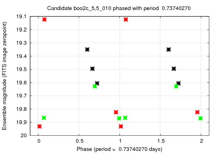
As an example, here is the "best-fit" phased light curve for a real RR Lyr star, as found by my stage 2 search:
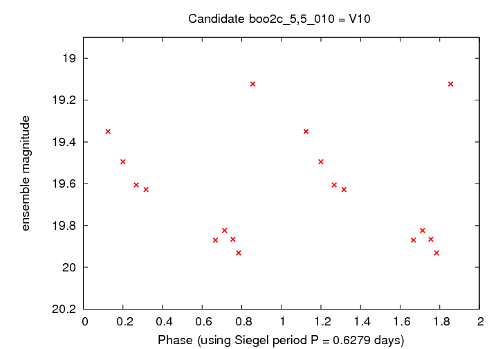
This is V10 from Siegel (2006). His (numerous) measurements show that the period is actually about 0.6279 days, rather than the 0.7374 days that my algorithm found. The light curve does look reasonable if one uses his period:
Since this stage of my search did not help, I would recommend that in the future
in order to improve the performance.