Quantitative consequences of zero-point errors in SNAP photometry

Michael Richmond
June 5, 2005

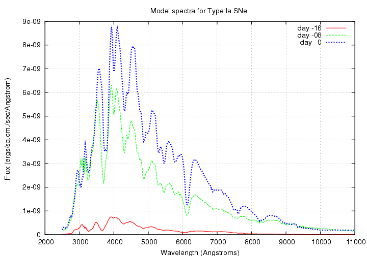
Ultra-quick summary: "the answer" (well, really just AN answer):

The goal is to find out quantitatively how small errrors in the zeropoints of the SNAP instrument would translate into errors in the cosmological parameters deduced from observations of SNe. I will describe a method of analysis which is somewhat different than the usual one, which I suggest may provide a useful secondary check on the usual methods.

For convenience, we assume that all Type Ia SNe are identical, and that we have a perfect model of their spectra at each point in their evolution. At a later time, we may incorporate a more realistic population of heterogeneous supernovae.

If there were no systematic errors ....

Now, suppose that there were no systematic errors in the photometric zeropoints of the SNAP instrument.

The inputs to the simulation factory

Supernova spectra over a range of ages around maximum light

We adopt the spectra of Type Ia supernovae provided by Alex Kim: http://snap.lbl.gov/bscw/bscw.cgi/d24909/snflux_1a.dat They cover the time range -16 days to +60 days after B-band rest-frame maximum light at intervals of 1 day, and the wavelength range 2,500 - 10,000 Angstroms at intervals of 10 Angstroms. Several examples are shown below:



Cosmological parameters

I chose a grid of values, with

  0.10, 0.11, 0.12, .. <  ΩM < .. , 0.49, 0.50 
  0.40, 0.41, 0.42, .. <  ΩΛ < .. , 0.89, 0.90
  

Overall instrument passbands

I used the nominal SNAP passbands first described by Alex Kim, based on redshifted versions of the Bessel B passband. You can look up the nominal transmission curves if you wish. One might use the overall transmission curves, which incorporate mirror and detector effects, in a future study.

Create simulated light curves

Given these inputs, we can create a set of light curves that the SNAP instrument would observe from supernovae at any particular redshift z. We do so in the following manner:

Choose SN redshift z

For reasons which will become clear in a moment, I restricted the initial tests to the range 0 < z < 1.0 . I then calculated the "proper-motion distance" for this redshift, which is the appropriate distance to use for a photon-counting instrument like the SNAP CCDs. The usual "luminosity distance" includes an extra factor of (1+z) for the change in flux due to the stretch in wavelength of each photon.

For each SNAP passband of interest

• compute rest-frame version of passband
• calculate the observed time of the spectrum (i.e., intervals of 1 day in the rest frame may turn into intervals of 2 days in the observed frame)
• convolve spectra with rest-frame passband to find the number of photons emitted through the rest-frame passband
• calculate observed instrumental magnitudes using the number of photons and distance modulus



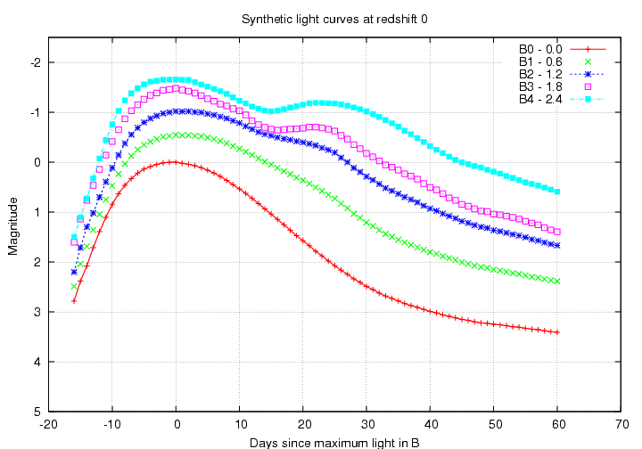
The input spectra cover the range 2500 to 10000 Angstroms. Over the redshift range z = 0.0 - 1.0, the SNAP passbands are shifted into the following ranges:

   SNAP filter     z = 0          z = 0.5        z = 1.0       
   --------------------------------------------------------
    B0          3600 - 5500    2400 - 3670    1800 - 2750

    B1          4200 - 6500    2800 - 4300    2100 - 3250

    B2          4900 - 7500    3270 - 5000    2450 - 3750

    B3          5800 - 8500    3870 - 5670    2900 - 4250

    B4          6000 - 10000   4400 - 6670    3300 - 5000
   --------------------------------------------------------
   

Filters B5, B6, B7, and B8 include wavelengths longer than the synthetic spectra in the rest frame, and so are disqualified from my initial study. Since filters B0, B1 and B2 are shifted out of the range of the input spectra at z = 1.0, I consider from here on the filters B3 and B4 only.

Find peak magnitude of each light curve

Next, we walk through all the input spectra and generate observed light curves for supernovae over the entire range of redshifts. For example, the B3 filter on SNAP (which is similar to the Johnson-Cousins I filter) will measure light curves like this:

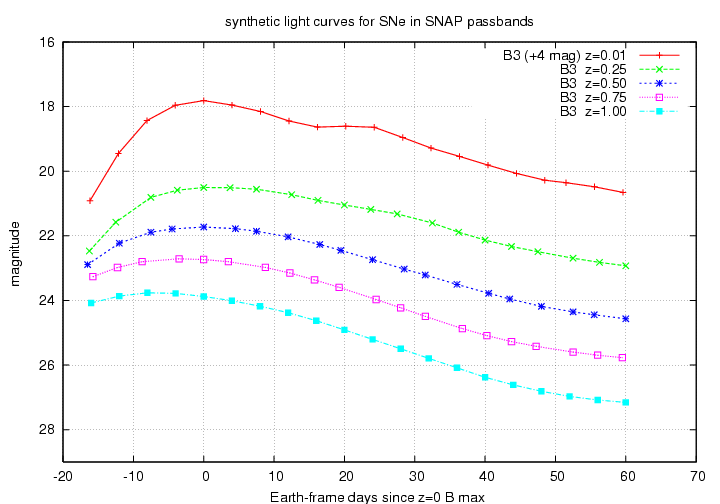
Note two different effects as the redshift increases:

1. A change in shape as filter samples bluer portions of the spectrum; the secondary maximum seen in nearby SNe Ia in the I-band disappears as the SNAP B3 filter becomes, in effect, an ordinary B-band filter around z = 1.
2. The stretch in time due to time dilation.

One can examine these observed light curves to look for the time of maximum light and its magnitude. I sampled the simulated light curves at both 1-day and 4-day intervals and fit cubic splines to find the peak values.

At this point, the usual procedure involves comparing the light curves in one filter at high redshift to the light curves in a different filter at low redshift, using the spectra to calculate K-corrections. I will now follow a different path ....

Build "the perfect Hubble diagram"

Now, given a sample of Type Ia SNe over a range of redshifts, we can plot the redshift and observed peak magnitude in some particular SNAP filter to create an observed Hubble diagram.

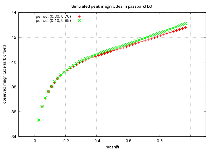
Both the shape and the location of the locus of peak magnitudes in this diagram tells us about the cosmological parameters Ω_M, Ω_Λ . The usual method of analysis concentrates on the location; that is, what is the peak magnitude of Type Ia SNe at a redshift of z=0.5, or z=0.7? This exact location along the vertical axis depends on several items which may contain systematic errors: the Hubble constant and the absolute flux calibration of the input spectra.

However, it is also possible to use the SHAPE of the locus, alone: measurements made by a single instrument which span a wide range of redshifts will indicate the proper cosmological parameters simply by the shape of the locus: one may shift the locus vertically by an arbitrary amount to find the best fit to a cosmological model. I will concentrate on this second method of attack. It is quite possible, of course, to follow both lines of analysis independently.

If systematic errors DO exist ....

One way to treat zeropoint errors in the photometry is as perturbations to the passbands, which translate into perturbations to the supernova spectra. For example, the statement "the B-band zeropoint is 0.02 mag higher than it ought to be" is equivalent to the statement "the overall B passband has transmission values systematically too low by two percent," which can be simulated by pushing the input spectrum values UP by two percent in the region of the B0 filter.

So, we can evaluate the effect of zeropoint errors in the following manner:

Modify the inputs:

• (same) Original supernova spectra over a range of ages around maximum light
• (same) Cosmological parameters Ω_M, Ω_Λ
• (modified) Perturb the overall instrument passbands, and propagate those changes into the input spectra. For example, we can simulate an error of 0.05 mag in the zero point of the B0 passband by multiplying all fluxes within the B0 passband by 1.05.

  

Create simulated light curves

We follow the same procedures as before; the only difference is the perturbed input spectrum for each day.

Find peak magnitude of each light curve

Build "the perturbed Hubble diagram" showing peak magnitude versus redshift

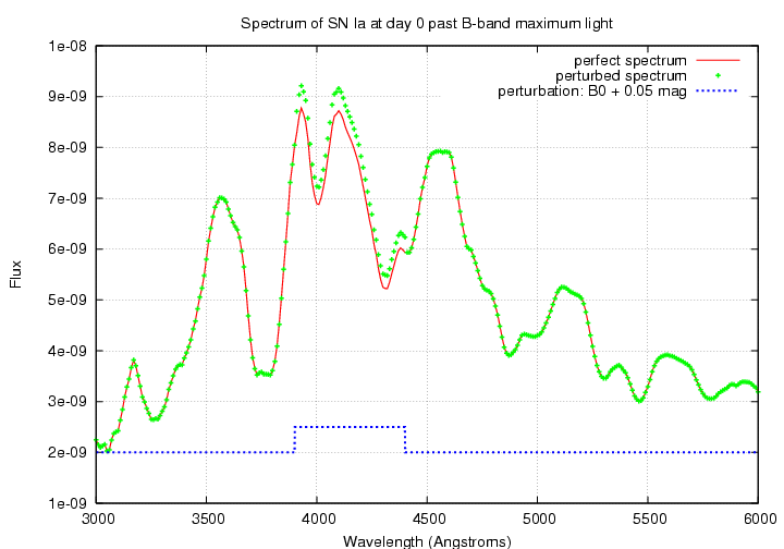
Now, unknowing astronomers on Earth will observe the perturbed Hubble diagram, but believe that it derives from perfect inputs. They will therefore compare the observed, perturbed peak magnitudes to their model, perfect peak magnitudes. We do the same:

Find the best-fit cosmological parameters

We compare the observed (perturbed) peak magnitudes as a function of redshift to a set of (perfect) model magnitudes as a function of redshift for a grid of values Ω_M, Ω_Λ . I allowed the observed magnitudes to slide vertically (i.e. we allow a small constant offset in magnitude) to account for errors in the Hubble constant or for errors in the absolute flux scale; I concentrated on the SHAPE of the observed locus alone to derive the cosmological parameters.

The difference between the true input parameters and those inferred from the match of observations to theory yields the desired output: the quantitative bias caused by any particular type of zeropoint error.

Results: samples of systematic errors

I have thus far tested the following specific examples of systematic errors:

• A: no errors, "perfect" system
• C: 5 percent boost at all wavelengths

• B: +2 percent change to QE over filter B0
• D: -2 percent change to QE over filter B0
• E: +1 percent change to QE over filter B0
• F: +5 percent change to QE over filter B0

• G: +2 percent change to QE over filter B2
• H: -2 percent change to QE over filter B2
• I: +2 percent change to QE over filter B4
• J: -2 percent change to QE over filter B4

• K: +2 percent change to QE over filters B0, B2, B4
• L: alternating +2/-2 percent change to QE over filters B0, B1, B2, B3, B4

• M: linear tilt in QE of +0.01 mag per 1000 Angstroms
• N: linear tilt in QE of -0.01 mag per 1000 Angstroms
• O: linear tilt in QE of +0.004 mag per 1000 Angstroms
• P: linear tilt in QE of -0.004 mag per 1000 Angstroms
• Q: unrecognized extinction of Av = 0.005 mag
• R: unrecognized extinction of Av = 0.010 mag

The results of simulations are shown in the tables below. I generated light curves for supernovae at redshifts 0.01, 0.03, 0.05, ..., 0.99. The noiseless simulations have a single event at each redshift; the simulations with noise place 5 events at each redshift, for a total of 250 SNe.

Recall that the input cosmology for the simulations had Ω_M = 0.30, Ω_Λ = 0.70. The entries in the table show the differences from these input values derived from fitting the perturbed observations of (z, peakmag) to the perfect model. For example, an entry in the table of

            -0.02  +0.05

Noiseless obs at 1-day intervals
case	filter B3		filter B4
	Δ ΩM	Δ ΩΛ	Δ ΩM	Δ ΩΛ
A	0.00	0.00	0.00	0.00
C	0.00	0.00	0.00	0.00
changes to B0 only
E	0.00	-0.02	+0.02	+0.02
B	0.00	-0.03	+0.04	+0.05
F	0.00	-0.07	+0.09	+0.10
D	0.00	+0.03	-0.04	-0.05
changes to B2 only
G	-0.01	+0.01	-0.05	-0.09
H	+0.02	0.00	+0.05	+0.09
changes to B4 only
I	0.00	+0.01	+0.02	+0.07
J	0.00	-0.01	-0.02	-0.07
changes to several filters
K	-0.01	-0.01	0.00	+0.01
L	+0.03	+0.04	+0.02	+0.05
linear tilt across spectrum
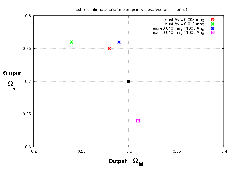
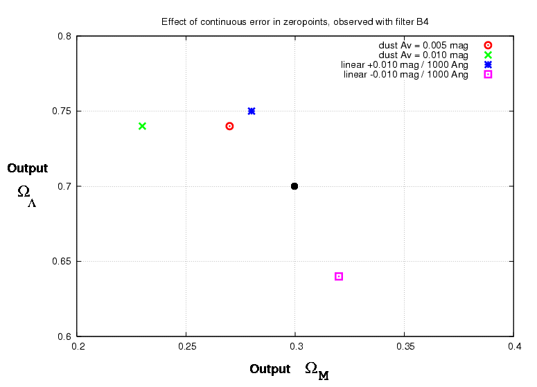
M	-0.01	+0.06	-0.02	+0.05
N	+0.01	-0.06	+0.02	-0.06
O	-0.01	+0.01	-0.01	+0.02
P	+0.01	-0.01	-0.01	-0.02
unrecognized extinction
Q	-0.02	+0.05	-0.03	+0.04
R	-0.06	+0.06	-0.07	+0.04

Noiseless obs at 4-day intervals
case	filter B3		filter B4
	Δ ΩM	Δ ΩΛ	Δ ΩM	Δ ΩΛ
A	-0.01	-0.01	-0.01	-0.01
C	-0.01	-0.01	-0.01	-0.01
changes to B0 only
E	-0.01	-0.03	+0.01	+0.01
B	-0.01	-0.04	+0.03	+0.04
F	-0.01	-0.08	+0.09	+0.11
D	-0.01	+0.02	-0.04	-0.04
changes to B2 only
G	-0.02	0.00	-0.06	-0.10
H	+0.01	-0.01	+0.04	+0.08
changes to B4 only
I	0.00	+0.01	+0.01	+0.06
J	-0.01	-0.02	-0.03	-0.08
changes to several filters
K	-0.02	-0.02	0.00	+0.01
L	+0.02	+0.03	+0.02	+0.06
linear tilt across spectrum
M	-0.02	+0.04	-0.03	+0.04
N	0.00	-0.07	+0.02	-0.05
O	-0.01	+0.02	-0.01	+0.02
P	0.00	-0.02	0.00	-0.03
unrecognized extinction
Q	-0.03	+0.04	-0.03	+0.04
R	-0.07	+0.05	-0.07	+0.04

The table below shows results for simulations in which a random error with RMS 0.03 mag is added to each measurement. Five events were generated at each redshift. As one might expect, the results are very similar to those for the noiseless simulation with the same 4-day interval.

Obs with RMS 0.03 mag at 4-day intervals
case	filter B3		filter B4
	Δ ΩM	Δ ΩΛ	Δ ΩM	Δ ΩΛ
A	-0.02	-0.03	-0.01	-0.02
C	-0.01	-0.01	-0.01	-0.02
changes to B0 only
E	-0.01	-0.03	+0.01	+0.01
B	-0.01	-0.04	+0.03	+0.04
F	-0.01	-0.08	+0.08	+0.09
D	0.00	+0.04	-0.04	-0.04
changes to B2 only
G	-0.02	0.00	-0.05	-0.09
H	+0.01	-0.01	+0.05	+0.10
changes to B4 only
I	+0.01	+0.03	+0.02	+0.08
J	-0.03	-0.05	-0.03	-0.08
changes to several filters
K	0.00	+0.02	0.00	+0.02
L	+0.01	+0.01	+0.01	+0.03
linear tilt across spectrum
M	-0.02	+0.05	-0.02	+0.05
N	+0.01	-0.05	+0.02	-0.05
O	-0.02	0.00	-0.02	+0.01
P	0.00	-0.03	0.00	-0.03
unrecognized extinction
Q	-0.03	+0.04	-0.04	+0.03
R	-0.06	+0.07	-0.07	+0.04

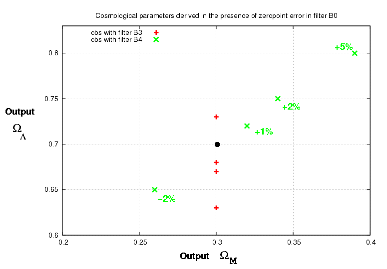
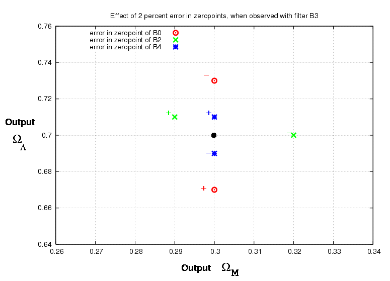
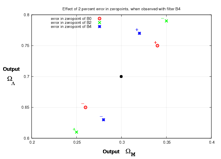
It may be simpler to grasp the general idea by looking at a graphical representation of subsets of the data. For example, suppose that there are errors only in the zeropoint of SNAP filter B0.

Note that the errors in Ω_Λ go in different directions, depending on the filter used to observe the supernovae. This is not always the case.

The next figure shows the effects of +/- 2 percent errors in the zeropoints of different individual filters:

• only an error in filter B0,
• or only an error in filter B2,
• or only an error in filter B4

Another type of error could occur all the way across the optical and near-IR spectrum. I simulated both a simple linear tilt, and extinction due to dust, which has a slight curvature as a function of wavelength.