We want to compare the apparent brightness nearby and distant SNe; deviations from the inverse square law tell us about the geometry of the universe.
Step 1
Here's how we do it:
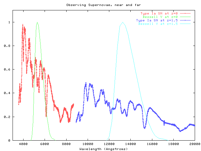
I(near) = (nearby SN spectrum) convolve (visual passband * QE_near)
I(far) = (distant SN spectrum) convolve (near-IR passband * QE_far)
The closer the near-IR passband is to a copy of the visible passband, shifted to the redshift of the distant SN, the better.
Step 2
Next, we make a second round of observations, using the same instruments to look at sources of precisely known spectra. We must know both the shape of each source's spectrum, and the relative brightness of each source.
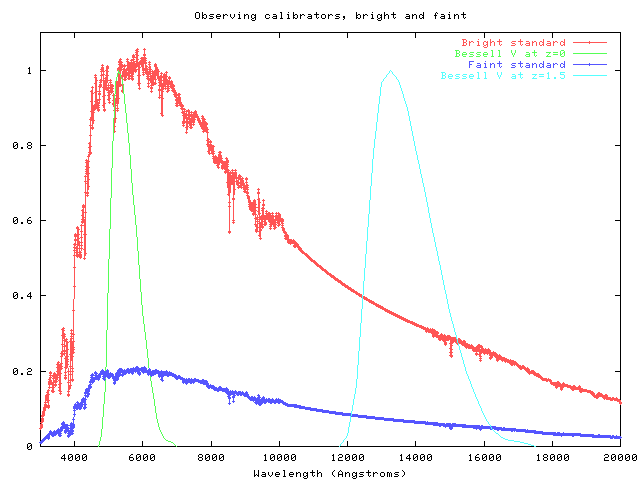
I(bright) = (bright known spectrum) convolve (visual passband * QE_near)
I(faint) = (faint known spectrum) convolve (near-IR passband * QE_far)
Step 3
We use observations of the standard source to determine the relative throughput, R, of the two instrumental systems:
              QE_far          I(faint)
            ----------  =  ---------------    =  R
              QE_near          I(near)
Step 4
Now that we know the relative throughput of the two instruments, we can compare the observed quantities fairly:
   I(far)        (distant SN spectrum) convolve (near-IR passband)
  -------   =   ---------------------------------------------------  *  R
   I(near)       (nearby SN spectrum)  convolve (visible passband)
Compare this ratio to the predictions of various models of the universe.
There are a number of mistakes which can lead to systematic errors and ruin the experiment. This is a partial list of them.
I will address here the first 4 issues only.
Shape of the instrumental passband
One can measure the spectral response of a filter easily; the response of a detector almost as easily; the response of a telescope with some difficulty; and the response of the Earth's atmosphere with much effort. A telescope on the ground has an effective passband which is the product of all these factors; in space, the response depends on the first three.
Instruments launched into space face a very different environment than that in which they were built. The change in temperature, pressure and humidity can cause the effective passband to change signficantly. The spectral response of the main detector on the Hipparcos satellite, for example, appears to have shifted to the blue by about 30 nanometers. The figure below, from Bessell, PASP, 112, 961 (2000) , shows the design passband (heavy dark line) and an estimate of the final, on-flight passband (narrow line to the left of the original).
If the actual passband doesn't match the assumed passband, how large is the resulting error in the photometry?
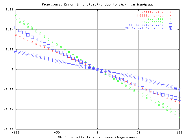
The figure above shows the fractional error in photometry (the convolution of a spectrum with a passband) as a function of a shift in the effective passband. I used two different filters:
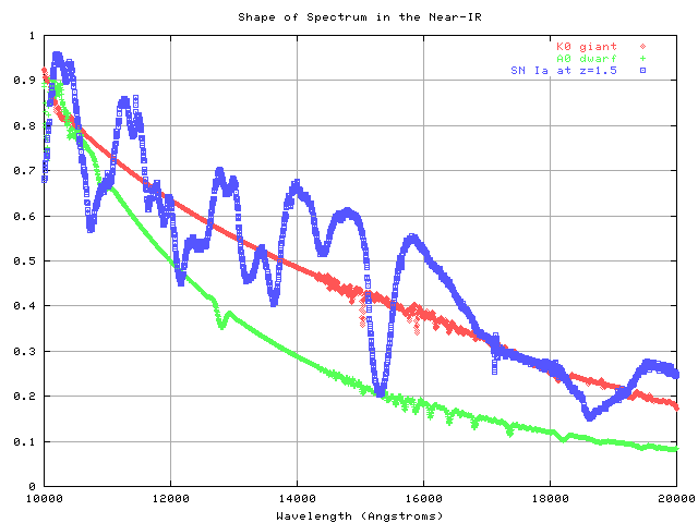
The figure shows the errors for three different stars: a "hot" star (A0 dwarf), a "cool" star (K0 giant), and a Type Ia supernova near maximum light at z=1.5. Note that
The differences between errors for stars and for the SN is due to the difference in their spectra: the spectrum of a Type Ia SN near maximum light is dominated by strong, wide absorption features. It is unlike the spectrum of any ordinary star.
Error in determination of SN redshift
If one makes an error in measuring the redshift of a distant SN, how large is the resulting error in the photometry?

One can calculate the fractional error in photometry for a supernova which is really at z=1.5, but is thought to be at some other redshift. In the figure above, I show the errors when observing through "wide" filters: versions of the Bessell B and V passbands, redshifted to z=1.5. The Bessell passbands have relatively gradual edges, especially on the red side. In the figure below, I show the errors when observing through passbands with relatively sharp edges: they are based on an interference filter, the SDSS i'. One is "wide" (central wavelength 13500 Angstroms, width 2100 Angstroms), the other "narrow" (central wavelength 13500 Angstroms, width 1200 Angstroms).
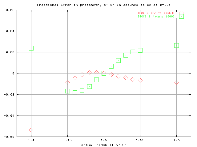
Note that an error of about 0.05 in redshift can lead to an error of 1-2 percent in photometry.
Error in relative scale of faint and bright standard sources
We will base the calibration process on a very bright fundamental standard star(s), which we will observe in a special manner (probably from a balloon-borne telescope, against a calibrated reference lamp). The fundamental standard(s) must be around magnitude 5, in order to gather enough photons in both the visible and near-IR to reach our required precision.
The nearby SNe will be roughly mag 12, a factor of about 630 times fainter.
The distant SNe will be roughly mag 25, a factor of about 100,000,000 times fainter.
We must transfer the calibration from the fundamental standard to fainter secondary, tertiary, etc. standards. Errors made at each step multiply together. If the faintest standard requires 4 transfers from the fundamental, and if the ratio of brightness is to be known to an accuracy of 1 percent, then each step must incur an error of no more than 0.25 percent, or roughly 0.0025 magnitudes.
Error in shape of standard sources' spectra
If the standard stars do not have exactly the same spectral shape, then we will calculate incorrectly the relative throughput of the instruments used to observe nearby and distant SNe. In order to prevent this effect from causing a 1 percent systematic error between the near and far measurements, we must know that the spectra of stars differing by 20 magnitudes in brightness are alike to 1 percent across the entire visible and near-IR.
We have argued elsewhere http://spiff.rit.edu/richmond/snap/primaries.html that the fundamental (and fainter) standard stars should be K giants. They
Our plan for the next six months is to do groundwork for the northern SNAP field, which we assume to be near the North Ecliptic Pole (NEP).
In the more distant future, we must