This document shows how I go through the process of turning ugly raw images from the RIT Observatory into the beautiful light curve of a variable star. I'll use a set of images of the cataclysmic variable star HS2331+3905 = V455 And taken by Joe Panzik on Sep 24/25, 2007 to illustrate the process.
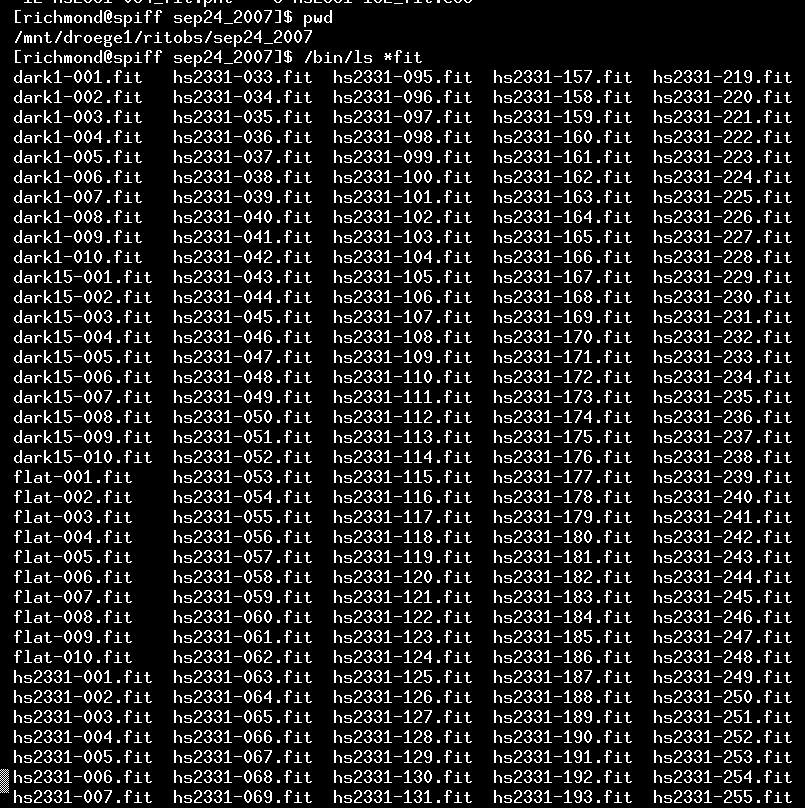
This is pretty easy: just copy the files into a directory somewhere. I'm going to use the directory called "sep24_2007" to reduce these images. Here is the start of a listing of the images.
Note that most of the images have names like hs2331-014.fit -- those are the images of our target object. There are also a few images with names like dark-001.fit and flat-001.fit -- those are calibration frames. I prefer to give the different types of images distinctive names, just to make it easier to identify them.
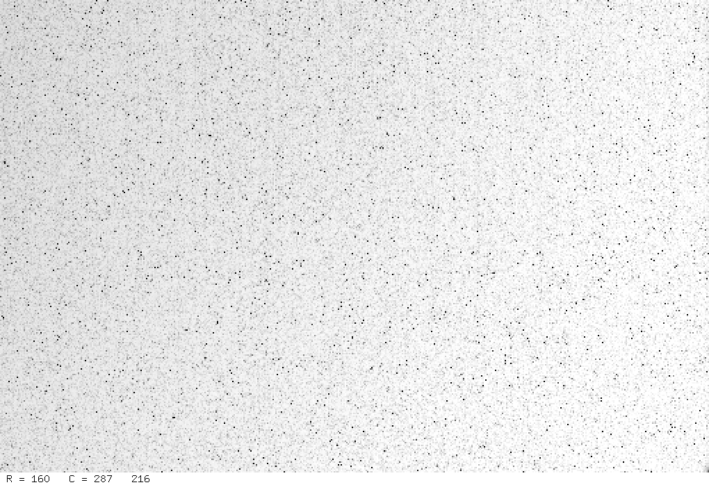
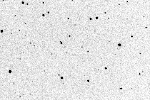
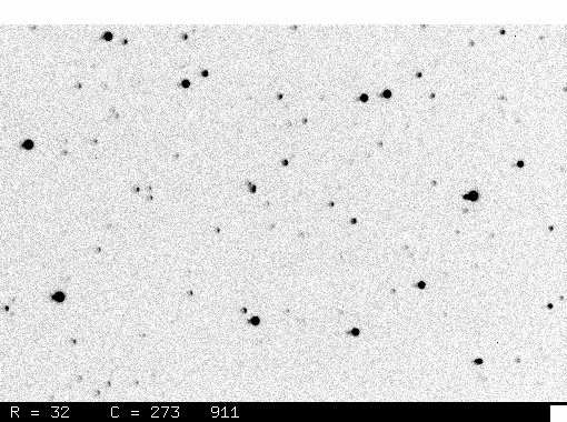
It never hurts to look at a few raw images, just to make sure that nothing funny was happening during the observing run. I'll look at one of the target images, number 276 in the sequence.
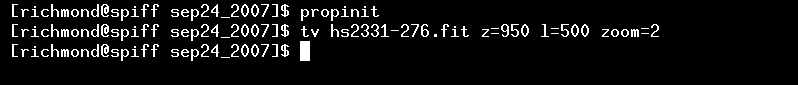
The XVista package has a command called propinit which needs to be run once, just to set up the computer's display. After that, I use the tv command (as I will a lot during this tutorial) to display the image on my computer's screen. I've arranged to use a "photographic negative" colormap, so that bright objects appear black and dark regions are white.
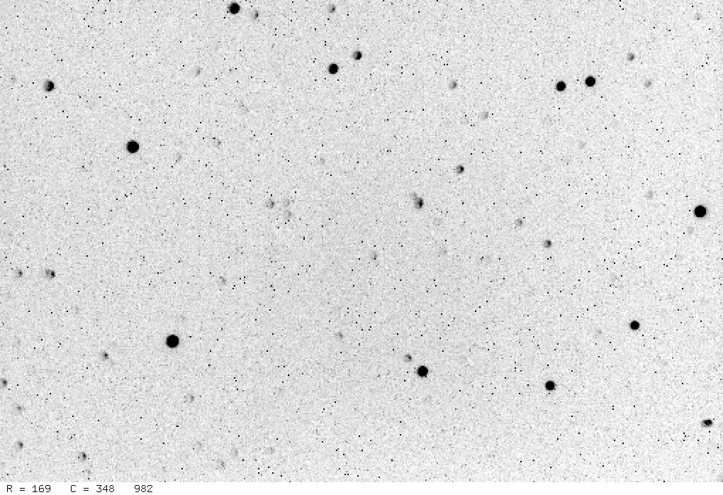
Yuck! This doesn't look too good.
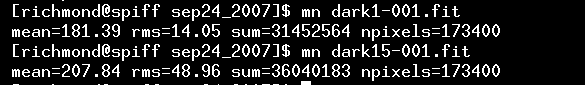
We have two sets of dark frames: one with 1-second exposure times (to be used with the 1-second flatfield frames), and one with 15-second exposure times (to be used with the 15-second target frames).
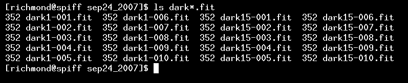
The signal counts of these frames are pretty low:
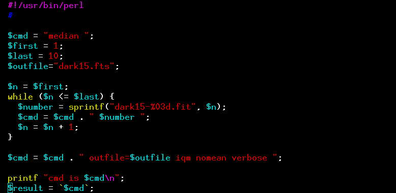
Now, the XVista command median will combine a number of images in the proper way: picking the median value at each pixel location. Using the median is more robust than simply calculating the mean value, since it will ignore outliers due to cosmic rays or other image defects. We could just type the median command with a long list of files as arguments -- as shown in this lecture -- but I've written a little Perl script to do the job. This makes the task quicker, because I can copy the script when I need to reduce another dataset; all I have to do is edit a few lines to change the filenames as needed.
Here's the first few lines of the make_dark.pl Perl script
or you can grab the entire script:
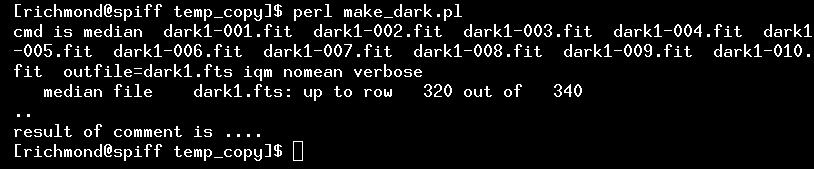
So, after I've edited the script to set the $first and $last and $outfile and $number variables to the proper values, I run the script like so:
I can examine the resulting output file, dark1.fts, by typing
tv dark1.fts zoom=2
which yields this image on my screen:
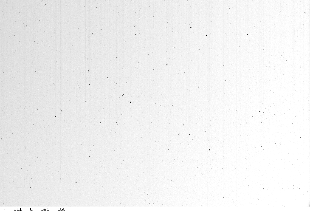
That's not very interesting -- just a few hot pixels on a bland, mostly level background. When I create a median dark from the 15-second dark frames, the resulting dark15.fts is slightly more interesting: it has lots and lots of hot pixels. No surprise -- there was more time for thermal motions to knock electrons loose.
Our next job is to create master flatfield frames. We have 10 raw flatfield images:
First, we need to remove the "dark current" from the raw flatfield images. To do so, we can subtract the 1-second master dark frame dark1.fts from each 1-second raw flatfield image. We could do this by typing a series of commands to the shell:
        sub flat-001.fit dark1.fts
        sub flat-002.fit dark1.fts
        sub flat-003.fit dark1.fts
        sub flat-004.fit dark1.fts

          etc.
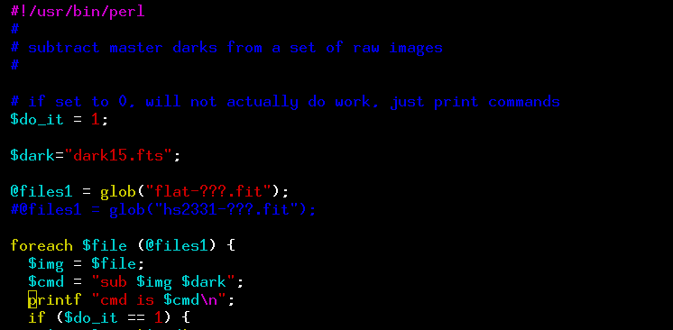
but it is quicker again to invoke a little Perl script to loop over all the raw flatfield images. Here's the first few lines of the sub_dark.pl script:
or you can grab the entire script:
I edit the script to make sure I'm subtracting the dark1.fts file from the files with names like flat-001.fit. Then I run the script by typing
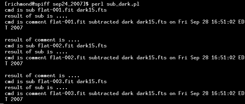
perl sub_dark.pl
which yields a long string of scrolling messages, starting like so:
The result is a set of flatfield images from which the "dark current" has been subtracted. We can then combine them to create a master flatfield image. The median command is again a good choice for the job; and, again, it's easier to modify a little Perl script than to type a long string of file names as arguments.
When I run the script, some informative messages appear:
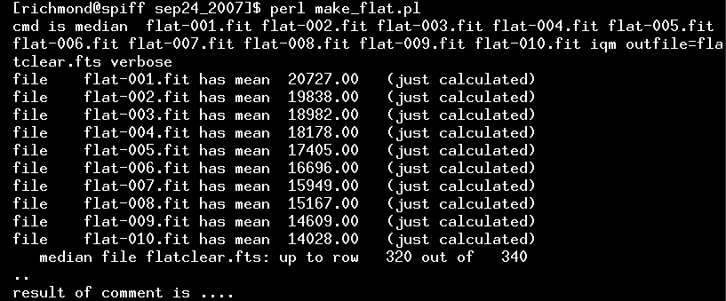
Those numbers are the mean values for each of the input images. Since Joe took the pictures after sunset, the brightness of the sky was decreasing pretty quickly. The median command will, by default, rescale all the input images so that they have same mean value, adjusting the later images to match the first one.
The result is a master flatfield image which is free of dark current and any stars that might have contaminated individual flatfield images.
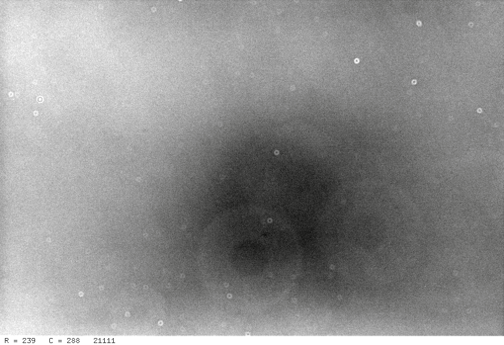
The small "donuts" are caused by diffraction around specks of dust which lie on the glass window just above the CCD chip in the camera; the large donuts are due to specks of dust on the surface of the "clear" filter.
As you can see in the report from Aug 2, 2004, flatfield images taken through different filters have distinct patterns, due to dust on the individual filters and to the change in sensitivity of the silicon with wavelength.
We are now ready to turn the raw target images into clean versions, via two steps:
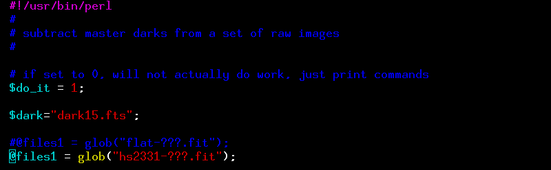
We can do the first step by editing the sub_dark.pl Perl script slightly, so that the proper dark frame and target frames are specified:
When we run the sub_dark.pl script, it prints out many messages as it processes the 276 target frames ...

Afterwards, each target frame looks better: the bright spots due to hot pixels are gone:
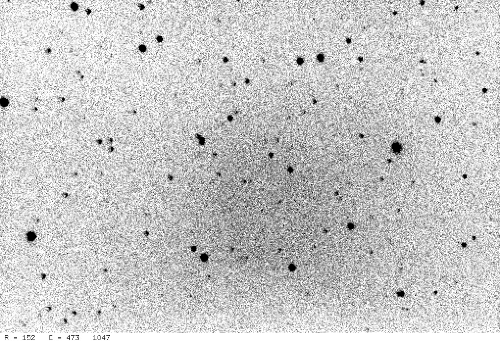
However, the center of the image is clearly brighter than the corners. If we divide by the master flatfield image, we should remove this pattern and leave a nice, uniform background all the way across the image. We could type one command for each of the 276 target frames:
div hs2331-001.fit flatclear.fts flat
but that would take a long time and be terribly tedious. It's much easier to have a little Perl script run through a loop over all the target frames for us.
Afterwards, we do see a nice, uniform background:

Now that the image has been cleaned up, it is time to locate the stars and measure their properties. We'll make use of two XVista programs to do these jobs:
We could run these programs directly, from the command line, but it would be a pain: there are many arguments for each program, and we might need to run the programs several times while figuring out the proper values for the arguments. Once again, I use short little Perl scripts: I can easily edit them to modify the parameters used as arguments, then run the programs without having to type them all from scratch.
Before we start, it helps to know the rough size of stars in our images. We can use one of the interactive features of the XVista tv command to find out. First, we display an image:
![]()
which causes a new window to pop up, showing the requested image.
When I move the cursor into this new window, the row and column coordinates of the cursor are displayed at the lower-left corner. I can zoom in on a star by moving my cursor to it and pressing the "z" key: a new window will pop up, showing a small subsection of the image at the cursor's location at a larger scale: For example, let me point to the bright star near the middle-right portion of the image and press "z".
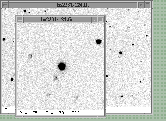
If I move the cursor to the center of this bright star and press the "r" key, another new window will pop up. This one will show a graph of intensity as a function of distance from the center of the star.

At the top of this graph are several pieces of information: the centroid of the star, its Full-Width at Half-Maximum (FWHM), eccentricity, position angle, and local sky value. The FWHM in this image is about 3 pixels; that's pretty typical for images taken at the RIT Observatory.
Okay, now that I know the FWHM of stars in my images, I can if necessary modify the Perl script which find stars.
At one point in this script, there's a line which contains the arguments to the stars command:
The current limits on acceptable stars are a minimum FWHM of 1.0 pixels, and a maximum FWHM of 6.0 pixels. My current images, with a FWHM of 3 pixels, should be just fine. But to be doubly sure, I'll make a limited test run first. At the top of the stars.pl script are a couple of lines like this:
By setting both debug and interactive to 1, I can cause the Perl script to do a little extra work: it will run through my images, one at a time, and for each one:
Here's what happens when I run the stars.pl script:
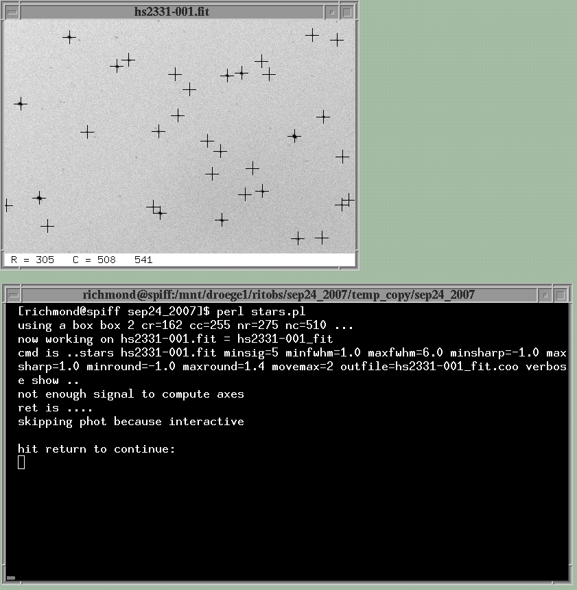
If the parameters are set properly within the Perl script, then all the obvious stars will be marked with crosses. That's clearly the case for this image, so I'm ready to stop messing around and process all the images. I go back to the stars.pl script and change the debug and interactive variables to zero.
It's also time to modify the parameters used for the second part of the job: measuring the brightness of each object. Near the bottom of the stars.pl script is a section which prepares to run the XVista phot program:
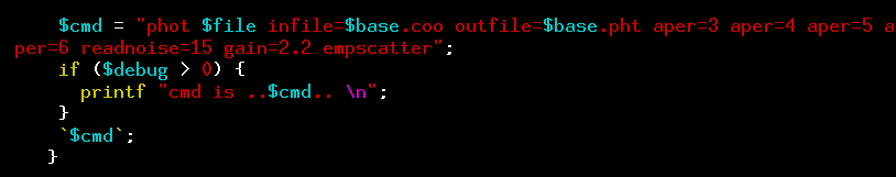
The code shown above will use circular apertures with radii 3, 4, 5 and 6 pixels to measure the brightness of each star; in other words, it will produce 4 different instrumental magnitudes for each star. That's not unusual -- it's often unclear exactly how large to make the aperture at this point, so we play it safe by making several measurements. We'll just pick the measurements we like best later on, and ignore the others.
Okay, we're ready to run the script for real. When it runs, you may see some messages scroll by in the shell window like this:
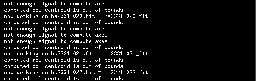
They are normal -- just ignore them.
After the script finishes, you should see a bunch of new files in the directory. For each image, there will be two new ASCII text files with similar names.
1 2.54 430.36 366 2.675 0.059 0.661
The columns are an ID number, row position, col position,
peak pixel value (after subtracting sky),
FWHM of the object, "roundness" of the object,
and "sharpness" of the object.
"Roundness" is a measure of the difference of the second
moments in each direction (zero means "round", +1 or -1
means "elongated), while "sharpness" is a measure of the
central pixel value to its neighbors.
the .pht files
1 2.54 430.36 996 8.42 16.009 0.038 15.939 0.045 15.944 0.055 15.933 0.064 4
The first three columns contain the object ID number, row position, and column position -- these will be the same for each object as the values in the .coo file. Next are the local sky value and uncertainty in that sky value. Starting in the sixth column are pairs of numbers: each pair contains an instrumental magnitude and an estimate of the uncertainty in that magnitude. In the line above, the measurements correspond to circular apertures with radius of 3, 4, 5 and 6 pixels, respectively. The instrumental magnitude is based simply on the number of counts (minus local sky) within the aperture:
instrumental mag = 25.0 - log10 (counts-sky)
The final column in the line is a "flag," which will be set to "0" if a measurement seems ordinary. Non-zero values, such as the "4" above, indicate that something may cause the measurement to be incorrect: the star might be close to the edge of the image, or it might be saturated, or have a close companion.
So, at this point, we have cleaned up all the images and created a list of the objects in each image, with positions and instrumental magnitudes.
We have a bunch of datafiles which contain the position and magnitude of each object detected in an image.
1 21.51 447.61 528 6.29 17.398 0.094 17.349 0.116 17.488 0.159 17.555 0.198 0
However, one piece of information that these files lack is the date and time at which the measurement was made. That's going to be very important a bit later, so let's add that missing piece to the datafiles.
The date and the starting time of each exposure are written into the header of each image; the format of these astronomical images is called FITS, short for Flexible Image Transport System . The format was created way, way back in 1981 by radio and optical astronomers. For example, here's a portion of the FITS header of one of our images, called hs2331-100.fit:

The camera opened the shutter for this image at UT 00:51:34 on UT September 25, 2007. The exposure length was 15 seconds. When we submit our photometry for publication, we need to report the middle time of the exposure. In this case, that would be about 8 seconds after the shutter opened, at UT 00:51:42.
The Perl script addheader.pl
Warning: the addheader.pl script calls two external programs which might not be on your system. The first is one called picksym, which picks out values from a FITS header. You should be able to grab and install this yourself from the bait package . The other is trouble: it is a command-line program called jd which calculates the Julian Date for some particular UT date and UT time. If this program isn't available on your system, you'll have to contact me for details.
goes through all the images taken during a night and pulls the date and exposure time from the FITS header; it then computes the midpoint of the exposure (by adding half the exposure length to the starting time) and converts the result into Julian Date . Finally, it appends the Julian Date to the end of every line in the star lists with photometry. So, an entry which originally looks like this:
1 2.54 430.36 996 8.42 16.009 0.038 15.939 0.045 15.944 0.055 15.933 0.064 4
will end up like this afterwards:
1 2.54 430.36 996 8.42 16.009 0.038 15.939 0.045 15.944 0.055 15.933 0.064 4 2454368.53590
So, when you are ready, you can run the addheader.pl script to insert a Julian Date to each line of all your photometry files.

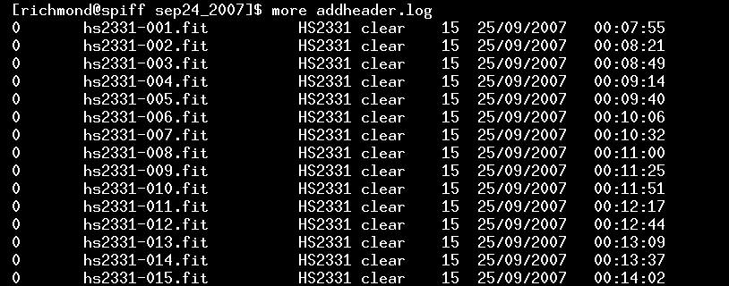
The script will print a bunch of lines for each file it processes. When done, there should be a new file called addheader.log in the directory. This is simply a list of the target images taken during the night:
All the modified photometry files, with the Julian Dates added to each line, will be placed in a new subdirectory; the original files are left as-is, in case you want to use them later on. The subdirectory in which the new versions are placed will have the name pff. So, after you have run the addheader.pl script, change directories into this subdirectory.
![]()
In this new subdirectory, there should be a bunch of photometry files with names like hs2331-010.pht, one file per target image.
It turns out that we can use some of the information from the star lists to make a quick check of the conditions during the night. For example, the background sky value near each star is listed for each image; we can make a graph showing that "sky value" as a function of time to identify times when clouds passed overhead.
I've written a little Perl script which looks through all the .pht files and .coo files for this sort of information. It must be run from the "pff" sub-directory.
This nightplot.pl script calls upon two auxiliary packages to do some of the work. They are both commonly found on *nix systems, but you might want to makes sure that they exist on your system before you try running the script.
If you can run the nightplot.pl script, you'll find that it creates three GIF images. The first, fwhm.gif, shows the Full-Width at Half-Maximum (FWHM) of the stars in each image. On this particular night, you can see that the width of stars increased during the night; that's due to a drop in the air temperature, causing the telescope to contract. One can re-focus every hour or so to avoid such changes.

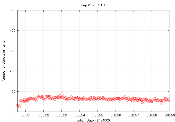
The second graph, numobj.gif, shows how many objects were detected in each image. In this case, the number was pretty consistent over the course of the run -- that's good.
The third graph, sky.gif, is perhaps the most useful. It displays the average sky background value as a function of time. On this night, the sky grew a little bit darker over the course of several hours after we started -- that's pretty typical. The jump at the beginning is due to a problem with the dome slit, I think.

Now, on some nights, the sky background will NOT show a smooth, gradual decline. If you see the sky value jump upwards, it probably means that some clouds were overhead.
Fortunately, this particular night seems to have been a pretty good one. Let's move on to ensemble photometry.
What is an ensemble? It is simply a large collection of stars observed on many consecutive images. Our goal is to use as many of the stars as possible in order to define the best possible photometric reference point on each image. The best reference for the following discussion is a paper by R. Kent Honeycutt published in PASP in 1992.
We are interested in the brightness of one particular star over the course of a night -- let's call it our "target star". Now, we could simply measure the instrumental magnitude of that star in each image, and then make a plot showing the instrumental magnitude as a function of time. If we were using a perfect instrument within a perfect environment, that would be fine. However, here on Earth, nothing's perfect: the atmosphere changes on timescales of minutes, clouds come and go, the moon rises, the temperature of our CCD camera drifts by a small amount. All these factors can change the overall sensitivity of our system, which will make the target star appear to vary -- even if it is actually remaining constant. Here's an example of a "light curve" produced during one night by this naive approach:
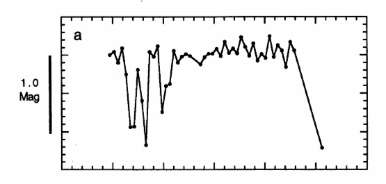
This figure taken from
Honeycutt's paper
It LOOKS as if the target star dropped over a magnitude several times during the first few observations, then brightened and remained nearly constant until the last measurement. But that's completely wrong -- all those variations are due to some clouds which drifted over the sky early during the night.
We can make a more accurate light curve if we perform differential photometry, measuring the difference between the brightness of the target star and a nearby comparison star on the same image. Most environmental factors will affect both stars equally, or nearly equally; clouds might make both stars dimmer by a factor of 10 -- but the ratio of the stellar brightnesses would not change. When we convert the intensities into magnitudes, that means that the difference in magnitudes would not change. Let's try that -- here's a graph showing the DIFFERENCE in magnitude between the target star and a single comparison star during the night.
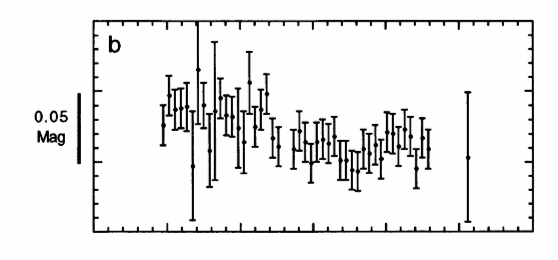
Notice how much smaller these variations are: the scale is now about 0.05 mag, not 1.00 mag. Differential photometry is a big improvement!
However, we can do better. If that single comparison star should turn out to be a variable source itself, then our differential light curve will a combination of the target star's changes AND the comparison star's changes. Yuck. Moreover, if a satellite or plane should fly past the comparison star, its brightness on one or two images might go way up -- which would make the brightness of our target star APPEAR to go way down. That's not good. It would be better if we used a group of comparison stars, instead of just one. That's what an ensemble is -- a group of stars which act all together to set the "mean level" against which to compare the light of the target. Below is a light curve of the target star compared to an ensemble of 25 comparison stars in a set of 38 images.

That's clearly better than the light curve using a single comparison star.
But there is one more (small) improvement we can make. The simplest sort of group is one in which all the stars appear in all the images; we can call that a "homogeneous ensemble." The calculations are pretty easy when we have measurements of every star in every image. But in real life, there are times when some stars don't appear in each imag: maybe the telescope tracking wasn't quite right, so some stars drifted out of the field of view; or maybe when clouds passed overhead, a few of the fainter stars disappeared; or maybe a satellite trail ruined the measurements of two stars in one of the images. In any of these cases, we would have to remove from our ensemble any star which didn't appear in even a single image.
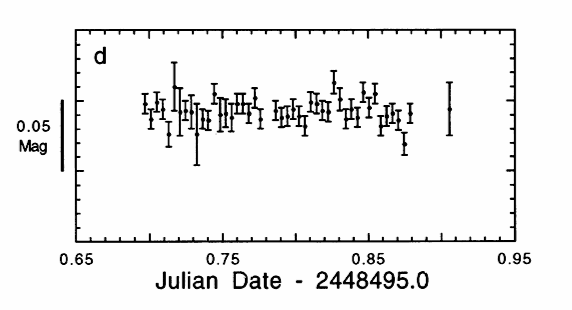
We would not have to discard any comparison stars if we could figure out a way to include stars which were missing from just a few images. In one image, we might have 26 comparison stars; in the next, 28 comparisons; in the next, 21 comparisons. By including all the stars we can see and measure from each image, we could maximize the statistical robustness of our ensemble; we might also be able to include some extra images in our analysis -- images in which only a few stars appear. Honeycutt provides a method for doing exactly this: using "inhomogeneous ensembles" of stars. I won't go into the details -- read his paper if you are curious. But take a look at the results: below is the final graph in the series, showing the light curve of our target star when it is compared to an inhomogenous ensemble of 92 stars in a set of 46 exposures.
Inspired by Honeycutt's example, I wrote software to put his method into practice.
We will use tools from this package to analyze our instrumental magnitudes in the following chapters.
We need to do some re-arranging. At the moment, we have list of stars arranged this way:
It will turn out later to be more convenient to have the measurements of each star collected together in one place, so that we have
It will also be convenient to discard some measurements entirely: false detections due to satellites or cosmic rays, real measurements of stars which only appear in one or two images with very low signal-to-noise.
The multipht program in the "ensemble" package will do all these jobs. It is possible to run it directly, but it requires a list of all the input star lists as arguments -- so you might have to type hundreds of words. I wrote a Perl script to add all the appropriate files as arguments, and to provide reasonable parameters to the program.
Let me explain briefly how you might modify this script. The important lines are shown below:
When you run this script, you should see a long list of lines start to scroll past, like this:
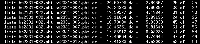
The file named in the second column is the "reference image" for the ensemble: it is used to define the "standard position" of stars. In this case, the reference image is hs2331-082. All other images are compared to this reference; their stars are shifted by some amount to match the positions in the "reference image." For example, we can see that the stars in image hs2331-007.pht must be shifted by 18.4 rows and 5.8 columns; when that is done, then 51 of a possible 55 stars match partners in the reference image.
After finding the shifts for all images, the program will present the user with three questions (advanced users may supply the answers in advance with extra command-line arguments -- see the ensemble manual ). The first question is how many stars must an image have to be included in the ensemble? If one particular image was taken during a cloudy period, so that it showed only 3 stars instead of 80 or 90, then it would make sense to remove it from any further analysis. To help the user make this decision, the program will print a table:
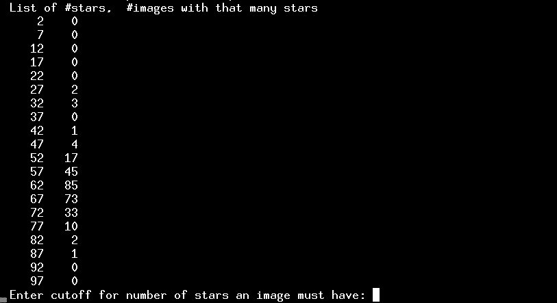
This indicates that most images had more than 50 stars. There are a few images in which fewer were detected -- two images, for example, had between 27 and 32 stars. However, no images were truly bad. I'll choose a cutoff of "20" -- which means that every single image will be represented in the final output.
The program now shows me a second table and asks a second question: in how many images must a star appear to be included in the ensemble?
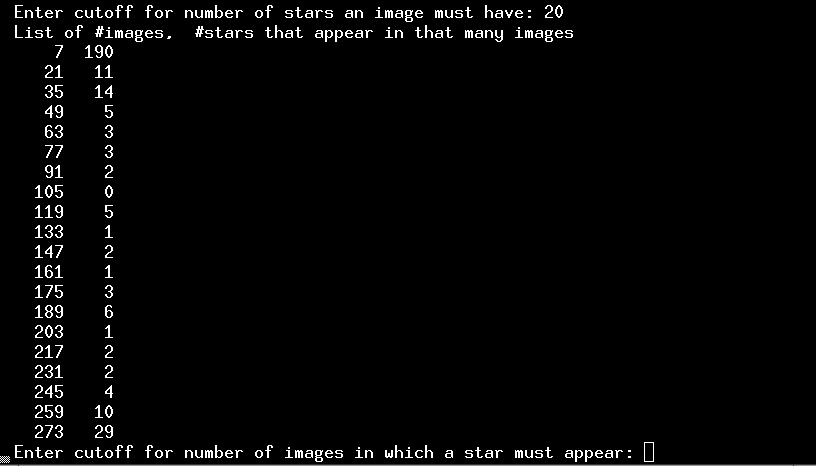
This table indicates the number of times a particular star was detected. My entire run consisted of 276 images, and 29 stars were detected in at least 273 of them. That's good -- those stars are surely bright, with decent signal-to-noise, and far from the edges of the pictures. Some stars failed to appear in a number of images: for example, 5 stars appeared in only 119 of the images. Why? They might be faint, falling just below the detection threshold in some cases; or they might lie close to the edge of the CCD, so that if the telescope drifted a small distance, they would fall outside the field of view. At the top of the table, we see that 190 "stars" were detected in fewer than 7 images. Most of these are probably not real stars, but false detections: cosmic rays, satellite trails, double detections in trailed exposures, etc. We definitely want to discard such garbage. Therefore, I'll set the cutoff to a large number: 50 images. If a source doesn't appear at least 50 times, it will not be included in the ensemble.
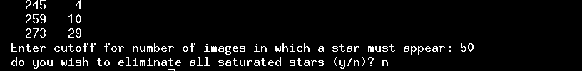
The third and final question is do you wish to eliminate all saturated stars? The earlier programs which created the star lists wrote a "status flag" into one of the columns. A zero in that column means "all is well", while a non-zero value means that something might be fishy: the star might be close to the edge of the image, or have a close companion, or have at least one pixel over some threshold for saturation. I recommend answering "no" to this question unless you are very familiar with your data and instrument and all the previous steps in the analysis.
Okay, we're done. The result should be a single very large text file which contains a record of every measurement of every star, all gathered together. In this example case, the file is called multi6_.out, and the first few lines look like this:
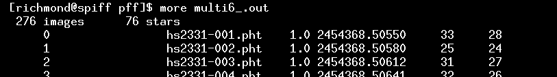
The very first line contains a count of the number of images and the number of stars in the ensemble. After that, the file has two basic parts:
If we scroll down to the end of this list of images, we reach the second part of the file:

It will be very handy to have a picture of the field with the ensemble star identification numbers printed next to each star. Let's make one. It isn't hard -- just three steps.
First, create a text file which contains one line for each star in the ensemble. The following Unix command will do that; remember that my big ensemble list is in multi6_.out. In this case, I'm creating a list of star positions called starpos_6.dat.
![]()
Next, display a picture of the "reference image" for the ensemble. As described in the previous section, my reference image is hs2331-082.fit.

Finally, run a Perl script called make_marks.pl with the name of the star position file as an argument.
perl make_marks.pl starpos_6.dat
As the script runs, little numbers will pop up on the window showing your image. Each number indicates a star's ID within the ensemble. In the example below, for example, star number 4 is very faint, and star number 28 is pretty bright.
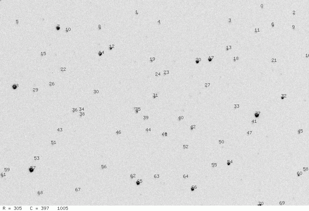
A warning: the little numbers are "fragile" -- if you minimize the image window and then expand it again, they will disappear. If another window sits on top of even a portion of the image window, then the little numbers may disappear when that overlying window is moved or closed.
I recommend strongly that you make a hardcopy of this image with the ID numbers superimposed. There are many ways to make a "screen grab"; just check your operating system.
In the chart above, the target star, HS2331, is star number 12.
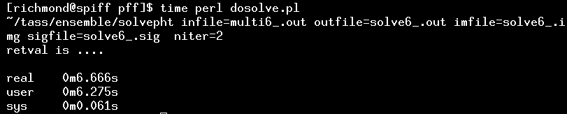
You are now ready to take the plunge and look for a global photometric solution to the entire ensemble of stars. The solvepht program within the "ensemble" package does this job. Rather than run it directly, I again recommend that you call it via a small Perl script.
It's especially handy to use a script for this task because you will probably run this step several times, making small changes to the arguments each time. The script will save you a lot of typing.
The solvepht program tries to find several quantities:
In my example, the input file is called multi6_.out. The output will consist of three files, with names
Depending on the number of stars and images in the dataset, this program may take a long time. In this example, with only 276 images and 76 stars, my computer needs only a few seconds:
Before we can publish the results, we ought to make sure that they make sense. There are several ways to examine the outputs of the ensemble solution which will tell us if something is fishy, or if the numbers really can be trusted. I have written a Perl script to put the quantities of interest into graphical form, using the same tools ( gnuplot and the ImageMagick suite ) mentioned earlier.
This script creates two graphs. The first, which has a name like emplot6_.gif, shows the "zeropoint adjustment factor" for all the images in the ensemble.

We see that at the beginning of the night, stars appeared fainter than they did at the end of the night; the size of the shift is about 0.4 magnitudes. This is a sign that I started taking images before the sky was truly dark. Once the sky did grow fully dark, though, at around JD 368.52, then there were no more major changes; the zeropoint remained steady to within 0.03 mag. That's the sign of a clear night.
On a cloudy night, the zeropoint will fluctuate up and down as clouds come and go. You can see some examples of these graphs on cloudy nights at
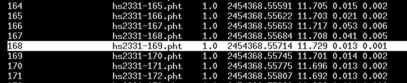
Sometimes there are isolated outliers in this graph; in my example above, the image taken at JD 368.55714 = hs2331-169 was shifted by about 0.3 mag relative to its neighbors. If I display that image, I see that indeed, something went wrong: each star has a small trail to the left. The tracking must have slipped for a moment.
When I examine the solve6_.img file, I see that this image had index number 168 in the solution --- that's the number in the first column on the left. I'm going to remember that; in a moment, I'm going to run the software again, telling it to discard this image from the ensemble.
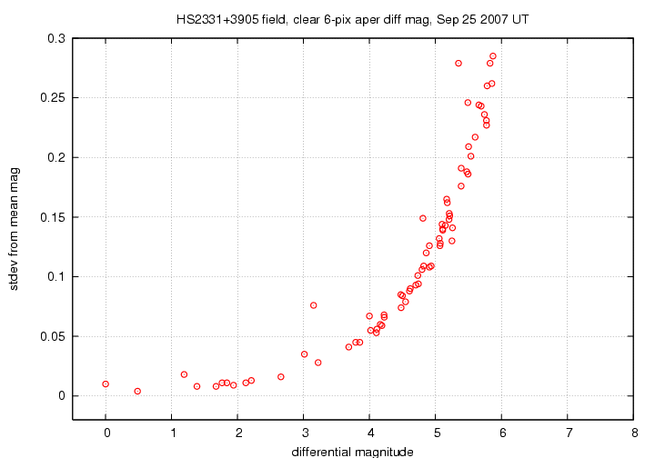
But first, I'm going to look at the other diagnostic graph, which has a name like magsig6_.gif. This shows how the uncertainty in the mean magnitude of stars increases from bright stars to faint ones.

Under ordinary circumstances, the brightest stars should have the smallest scatter, and the faintest stars the largest scatter. The graph above shows the proper trend, in general, but there's something fishy about the very bright end: the scatter seems a bit high. One reason this can happen is that the very brightest stars in the image might be saturated. If so, then their measurements are incorrect ... yet, because they are so bright, their measurements carry a large weight in the ensemble solution. One way to check for this unhappy situation is to mark the brightest star(s) as "variable", which will remove their influence on the overall solution.
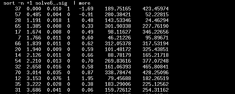
Which stars are the bright ones? The solve6_.sig file will tell me if I sort it properly:
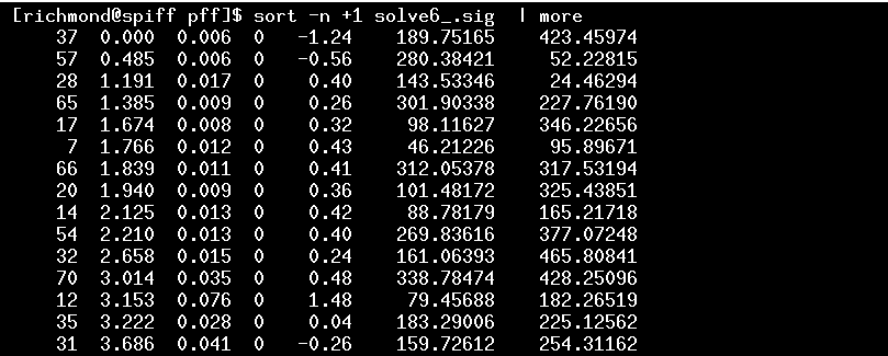
The very brightest star is number 37, which lies near position (189, 423) in the image. The finding chart shows me that this star is indeed very bright, so it's reasonable that it might be saturated. The third-brighest star, number 28, has a scatter which is a big larger than its nearest neighbors; when I examine all the images carefully, I see that it fell near the very edge of the CCD chip at times, when the telescope drifted a bit to the West. I ought to get rid of star number 28 -- its measurements are contaminated by a few bad ones. I also notice that the target star, HS2331, number 12 on the chart, has a large scatter: its symbol, at differential magnitude 3.15, lies far above the locus of other stars. Since I know that this object is varying, I should mark it in some way, too, so that it doesn't throw the solution off.
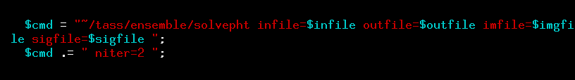
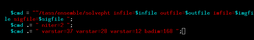
I will edit the dosolve.pl script to make three changes: I will remove the trailed image, number 168, from the solution, and I'll mark stars number 37, 28 and 12 as possible variables, so that they don't ruin the measurements of other stars. This is what the important section of the original version of dosolve.pl looked like ...
... and this is what it looks like after I insert a few new lines to take care of the bad image, the known variable target star, the saturated star, and the star near the edge of the chip.
You can read the the ensemble manual for details on the arguments of the solvepht program.
Having modified the dosolve.pl script, I run it again.
If all went well, the solution ought to look better this time. Does it? I make a second round of graphs using the solplot.pl script. Here they are: the graph of zeropoint adjustment factors no longer shows the outlier in the middle of the run:

The scatter-vs-mag graph does indeed look a little bit better: now the second-brightest star has a smaller scatter than it did earlier.
If I sort the new solve6_.sig file to show the brightest stars again,
you can see that the stars I marked as "varstar" now have a "1" in the fourth column. You can also see that the second-brightest star now has a scatter of only 0.004 mag from its mean value; in our first run, its scatter was 0.006 mag.
Hooray! At this point, you have all the information you need to make a light curve for the target star (or other stars in the field). The main solvepht output file consists of a number of "stanzas"; each stanza provides the measurements of a star throughout the run of observations.
For example, here are the first few lines of my copy of solve6_.out.
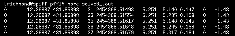
As you can read in the ensemble package manual, the columns mean
The most important of these are columns 5 and 7: they yield the time and magnitude for each measurement. In this example, I have managed to put Julian Date into the "time" column; if you didn't have access to FITS headers or some other source of Julian Date, your ensemble might have a set of index numbers in the "time" column -- making it the same as the "image index number". Note that since the Julian Date has values which are very large, like 2454368.54232, the labels on the horizontal axis of a graph may run into each other and be hard to read. For convenience, when I make a graph, I will subtract a big constant, creating a "truncated" date which is easier to write and say.
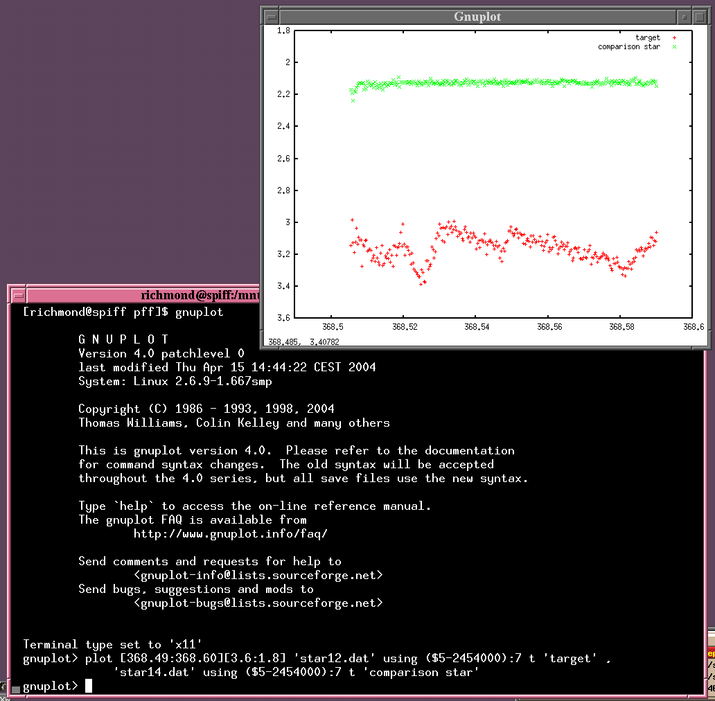
So, if I make a graph with column 7 on the y-axis and column 5 on the x-axis, I'll have a light curve of an object.
Whoops! Don't forget that when plotting magnitudes, put small numbers at the top and big numbers at the bottom.
In order to pick out the measurements of a single object, I need to extract its lines from the file. In this example, the target star was object number 12, while a nearby comparison star was number 14. So, here's a simple way to make a graph.

My choice is gnuplot .
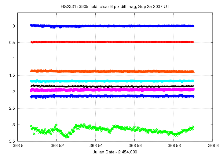
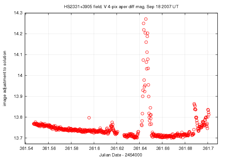
When I write up my results for a night of photometry on some specific target, such as for the night from which this example was taken , I like to make two graphs with light curves. The first shows a sample of bright and faint stars over the course of the observing run, to give the reader some idea for the quality of the measurements across the range of stellar brightness.
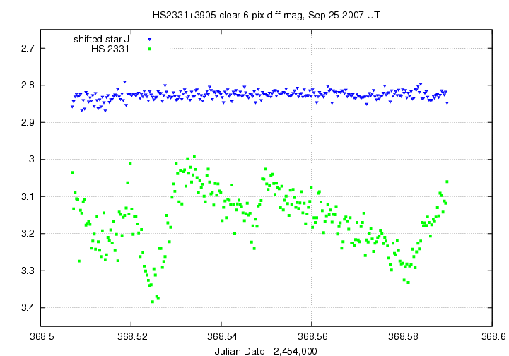
I also make a "close-up" light curve, showing the target and only a single, representative comparison star of similar brightness. This gives the reader all the gory details.
You can look at my Perl scripts for these graphs -- perhaps they give you some ideas for making your own graphs. Note that I use gnuplot to generate a Postscript file for each graph, then use the ImageMagick program called convert to turn the Postscript into a GIF image. I find that this yields more pleasing text and symbols than generating GIF or PNG images directly.