 Copyright © Michael Richmond.
This work is licensed under a Creative Commons License.
Copyright © Michael Richmond.
This work is licensed under a Creative Commons License.
You can find this talk at
http://spiff.rit.edu/richmond/asras/subaru_pm/subaru_pm.mar2009.html
During the spring of 2008, I spent two months at Institute of Astronomy in Tokyo, thanks to a fellowship from the Japan Society for the Promotion of Science. While I was there, I worked with a group of astronomers,
Contents
The Subaru Telescope, run by the National Astronomical Observatory of Japan , is one of the largest in the world. Its primary mirror is a single piece of glass, 8.2 meters in diameter.
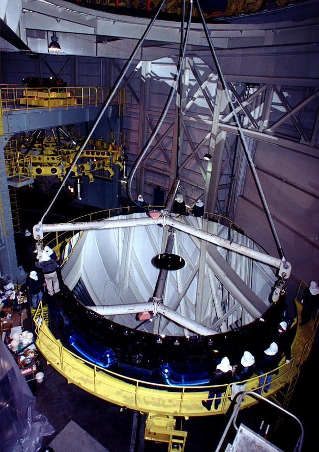
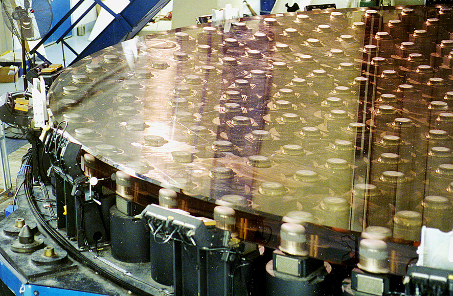
To keep this thin piece of glass from bending or warping, which would change its shape and throw images out of focus, there is a very complicated active support structure beneath it:
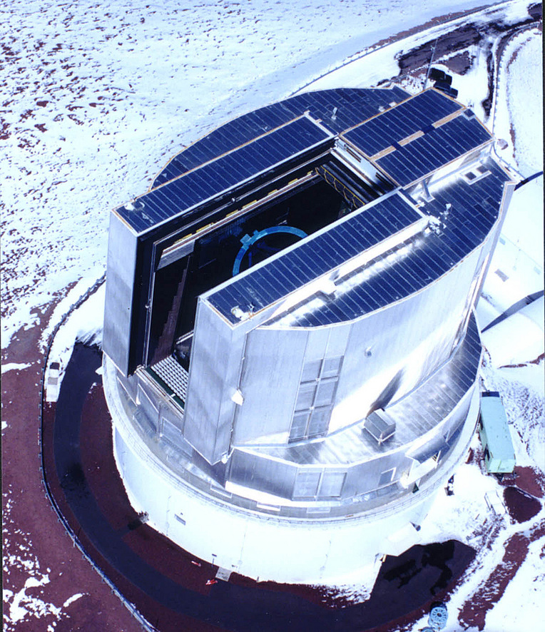
The telescope sits high atop Mauna Kea, at an altitude of 4200 meters above sea level. The entire enclosure rotates with the telescope to follow the stars.
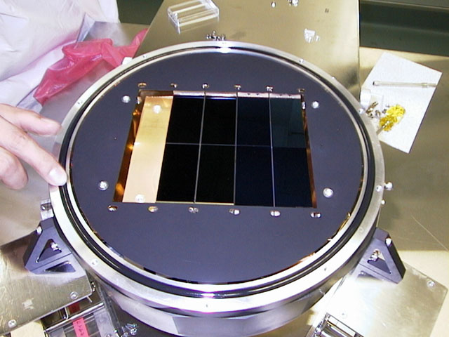
The size of the field is just about the field of view of one of the main Subaru telescopes, the Suprime-Cam. This optical camera has 10 CCD chips, each 2048x4096 pixels in size, arranged in a 2-by-5 array. At the prime focus of Subaru, it provides a field of view of 34 by 27 arcminutes. Each exposure yields a raw image 160 MB in size, so it's not trivial to do the data reduction ...
The SDF team has taken images of this field in seven passbands: five are wide filters, B, V, Rc, i', z', and two are narrow-band filters used to look for certain emission-line objects, NB_816 and NB_921. In order to fill in all the gaps between the CCDs, the operators take a series of short exposures -- each about 300 seconds long -- with small offsets in position between each. Each passband accumulates 1-3 hours of exposure time per epoch. The result is a large area of very deep images, reaching point sources down to magnitude 26-28.
The combination of Subaru + Suprime-Cam yields images which cover quite a large region of the sky (from an astronomer's point of view).

The combination of wide area and faint magnitude limits means that the SDF samples the stars in a very large volume of space. The table below compares it to several other surveys for proper motions. I've chosen the magnitude of faint, old white dwarf, Mv = +16.5, to define the distance out to which each survey reaches.
Moreover, the SDF project has accumulated up to 18 epochs of measurements for each star, compared to just 2 or 3 for many proper motion studies. That means that we should be able to reduce the number of false positives to levels far below those of some surveys. This is especially important when one is studying faint objects near the limits of detection.
Subaru is a general-purpose telescope, with several different instruments. Many astronomers apply for time on it and point it at different objects. However, the allocation committee has given large blocks of time to several big groups so that the telescope can carry out big projects which can support many different research activities. One of these is the Subaru Deep Field. The SDF is a region about half a degree on a side, located at high galactic latitude so that it suffers little extinction from dust in the Milky Way. Its center is at
        (J2000)    RA = 13:24:38.9   Dec = +27:29:25.9

                    l = 37.6           b = +82.6
which lies just inside the boundaries
of the constellation Coma Berenices.
There is another special region of the sky which has been observed not only in the optical, but also in the radio, X-ray, and infrared portions of the spectrum. This is the Subaru/XMM-Newton Deep Survey (SXDS) site .
It appears in the night sky during the autumn and winter.
Basically, these two regions lie in opposite directions, one above the plane of the Milky Way, and one below. This isn't an acccident: both regions were originally chosen in order to study distant galaxies, which would be blocked by dust in our Milky Way if we tried to look along the plane of the disk.
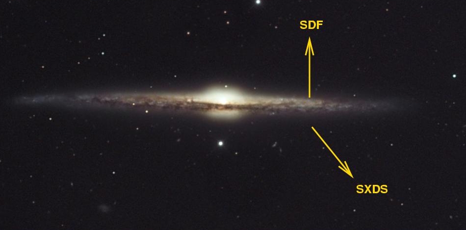
Image courtesy of
Robert Gendler
The basic idea is pretty simple:
Let's walk through this idea, one step at a time.
We started with a single seamless mosaic image from each epoch, created from several, dithered, individual exposures. We chose to use i'-band images because some of our likely targets would be relatively cool and red. We used a simple method(*) to detect point sources in each image and measure its brightness through circular apertures.
(*) the stars and pht programs from the XVista package
Since we didn't care about galaxies, just stars, and since we also were more interested in POSITIONS than magnitudes or other properties, this simple procedure was good enough.
The result was a list of between roughly 20,000 and 120,000 objects for each epoch -- more when the seeing was good and the total exposure time was longer.
Did we find every star in that region of the sky? No, of course not: we only noticed the bright ones. In order to quantify this important fact, I added artificial stars to the images and ran our routines to detect and measure the stars. We found nearly every bright artificial star, but only a small fraction of the faint ones. This tells us our efficiency as a function of magnitude, and gives us a simple way to describe the completeness of our search.
We broke up these very large lists into smaller pieces by dividing the area of the SDF into a regular grid of 9-by-11 square sections. Each section was about 1000 pixels on a side, with a small extra amount for overlap between neighboring sections. In part, we did this simply to make the subsequent processing easier; but it also helps to reduce the effects of any large-scale spatial distortion across the focal plane: we will be comparing the position of each star to its neighbors, rather than to objects half a degree away.
We then used the match package to compare the objects in this section to objects in the same section in the fiducial epoch: UT 2007 Feb 15. We allowed for a general linear transformation (translation, rotation and scaling) between the two lists of objects. The maximum permitted matching distance between an object in the two epochs was 5 pixels, which corresponds to about 1 arcsecond. Given a maximum six-year difference in time, this places an upper limit of about 0.17 arcsecond per year in the proper motion we can detect.
We looked at the position of each star in the row and column coordinates separately. For each direction, we fit a straight line to the positions as a function of time. Our fitting routine provided both the slope of that line, and a value for the uncertainty in the slope. In order for a star to pass this test, the ratio
                           slope of line
       significance  =  --------------------
                         uncertainty in slope
had to be large in either one of the directions, or in a combination of the two directions. Below is an example of one of the candidates which passed this test.


We accepted any star which had a combined significance level which corresponds roughly to "10-sigma". That led to 110 candidates.
After examining each candidate by eye, we discovered that five of them were spurious, due to the combination of light from several sources. That left 105 candidates with large proper motions .
Below are three examples of our candidates.
As a check to our procedure, we can look at the distribution of "motions" for objects which have a high significance -- such as the set of 105 solid candidates -- and those of low significance. Stars which don't really move, but simply have random errors in their measurements, are equally likely to have spurious (small) apparent motions in all directions. And, indeed, they do:

On the other hand, stars which are really moving ought to show some signature of kinematics in the Milky Way. The Sun, for example, is revolving around the center of our Galaxy in a circular orbit at about 200 km/s; halo stars, on the other hand, do not share this circular motion. Therefore, we expect to see halo stars zoom past us in one particular direction; that direction depends on which way we look. We called upon the excellent Besancon stellar population synthesis model to tell us which direction we should EXPECT stars to be moving.
We generated several random instances of stellar populations in the direction of the SDF, then picked those objects which fell into the magnitude and color limits of our survey. The resulting collection of simulated stars showed a pronounced asymmetry in their proper motions as seen from the Sun ... and we see that same asymmetry in the actual observed proper motions. This confirms that we are detecting real moving stars.
What can we say about these stars with high proper motions? Well, the the SDF catalog provides magnitudes for each object in five wide passbands. We can, in theory, use these measurements to calculate the colors of each candidate, which in turn might tell us something about its physical properties.
Unfortunately, some of the candidates are very red. They show up clearly in the i'-band images we used to search for proper motion, but they do NOT appear in images taken at shorter wavelengths, such as B-band. Of the 105 candidates, 6 were so red and faint that we could not extract reliable B or V magnitudes. We discarded those objects, leaving 99 candidates with reliable motions and colors.
One of the astronomer's most useful tools is the color-magnitude diagram. If we know both the color and the absolute magnitude (or luminosity) of a star, we can tell if it is still on the main sequence and burning hydrogen, or if it has moved into a later evolutionary stage.
Image courtesy of anzwers.org
Unfortunately, in order to determine the absolute magnitude of a star, we need to know its distance. We do not know the distances to our candidates in the SDF, and so we can't place them onto a color-magnitude diagram.
However, there is something we can do. We can use their motions as proxies for their distances. To some extent,
Astronomers who use proper motions long ago (in 1922!) came up with a mathematical expression which replaces the distance d to a star with an expression based on its apparent proper motion μ.
The quantity H is called reduced proper motion. We can use it in place of absolute magnitude to make a graph analogous to the color-magnitude diagram. In this reduced-proper-motion diagram, the position of a star isn't identical to its position in the color-magnitude diagram ... but we can still distinguish between different types of stars. I'll first show a version of this diagram with synthetic model stars only, to give you an idea of what we might expect to see.
As you can see, stars belonging to different populations will tend to fall in different regions of the reduced-proper-motion diagram. In particular, the left side of the lower portion is the domain of white dwarfs: stars which are relatively hot (and therefore blue), yet very low in luminosity.
Now, let's plot our 99 candidates on this sort of diagram. In order to reduce confusion, I'll use tiny dots for all the stars in the synthetic model, and big squares with errorbars for the 99 real candidates.
Many of our candidates fall into the "halo" region of the diagram, suggesting that they are main-sequence stars in the halo of the Milky Way. There are a few candidates in the "white dwarf" region. But what about the bunch which lie in the angle between the "white dwarf" and "halo" regions?
Well, that's a good question. There are several possibilities:
What are sub-dwarfs? They are stars which are burning hydrogen to helium in their interiors, like ordinary dwarfs, but which have a different chemical composition: their outer atmospheres have a lower content of "heavy elements" such as carbon, iron, silicon, etc. They are called "sub-dwarfs" because in an ordinary color-magnitude diagram, they appear underneath the ordinary dwarfs. Or, put another way, they are bluer than regular dwarfs of the same luminosity.
Please note that we're not sure that the stars with high motions and intermediate colors are REALLY sub-dwarfs; we would need to take spectra of them to be positive. Unfortunately, most of these stars are so faint that acquiring good spectra would take a lot of telescope time....
At the moment, I am working my way through the SXDS dataset. I haven't finished, but some preliminary results show the same pattern as the SDF: we find some objects which are likely to be white dwarfs, and others which might be halo subdwarfs.
There are four things we can (and will) do to continue our study of moving stars:
We'll be applying for time on Subaru to make these observations soon: the deadline for Spring 2009 observing is in September, 2008.
Rejected
There are 72 objects with slightly lower levels of significance to their motion: 4.0 < Stot < 5.0. Many of these objects, perhaps the majority, will also turn out to be real moving stars. We simply need to look at each one closely.
On the back-burner ...
It is also possible, though unlikely, that there might be some very distant objects belonging to our own solar system in these images. The ecliptic latitude is 33 degrees, which is high, but perhaps not too high. We would have to make a special kind of search with new procedures to find solar system objects, since they would move very rapidly. However, if we examined only the images taken during one season at a time, without requiring nearby matches in images from other years, we might find something ...
On the back-burner ...
In progress
Copyright © Michael Richmond.
This work is licensed under a Creative Commons License.