 Copyright © Michael Richmond.
This work is licensed under a Creative Commons License.
Copyright © Michael Richmond.
This work is licensed under a Creative Commons License.
I'm reporting on work which involves other people:
Table of contents
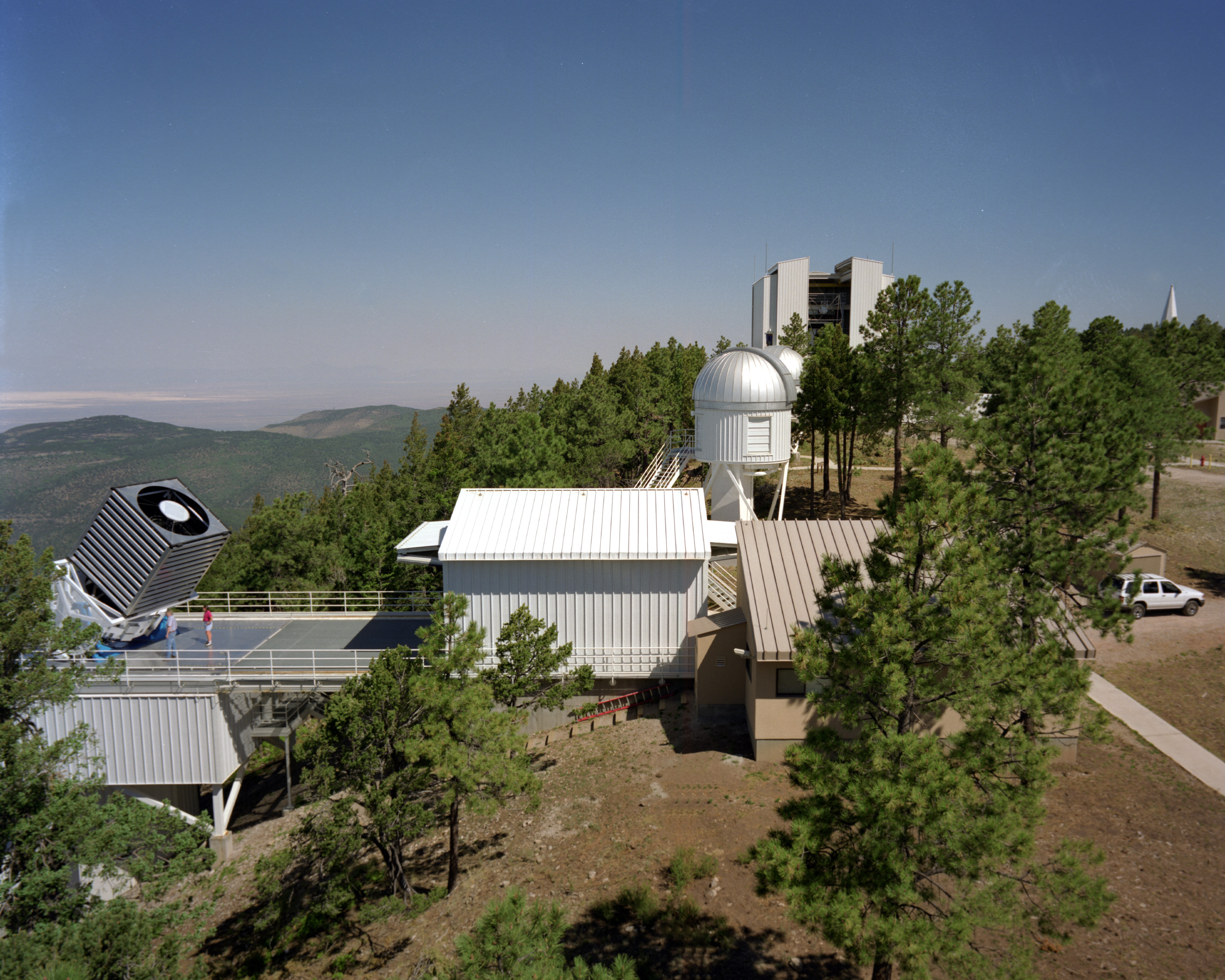
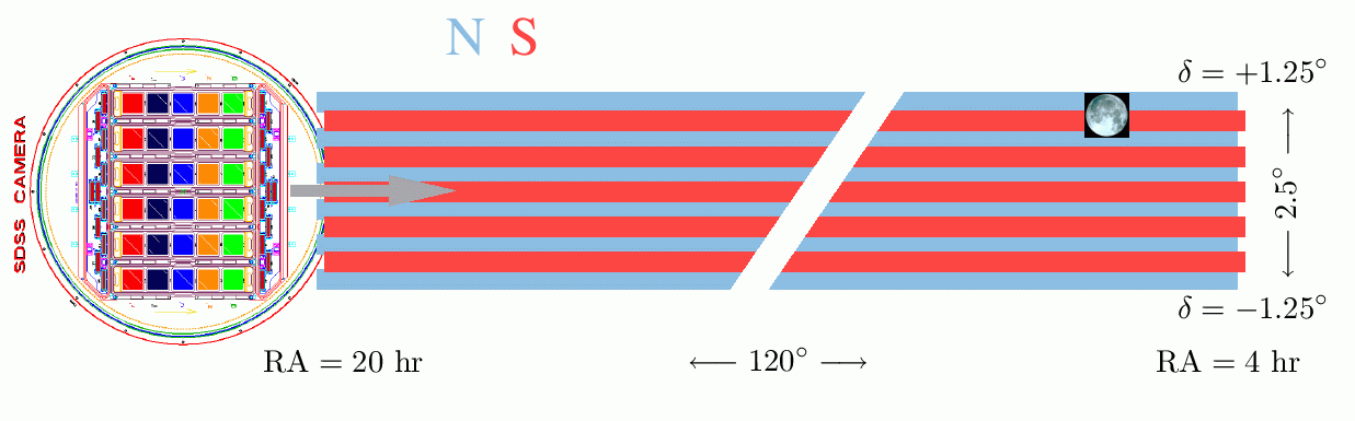
The main telescope has a telescope 2.5 meters in diameter. It sits out on a track, away from the face of the mountain, so that the prevailing west winds will sweep across the telescope smoothly before the ground and trees stir up a lot of turbulence.
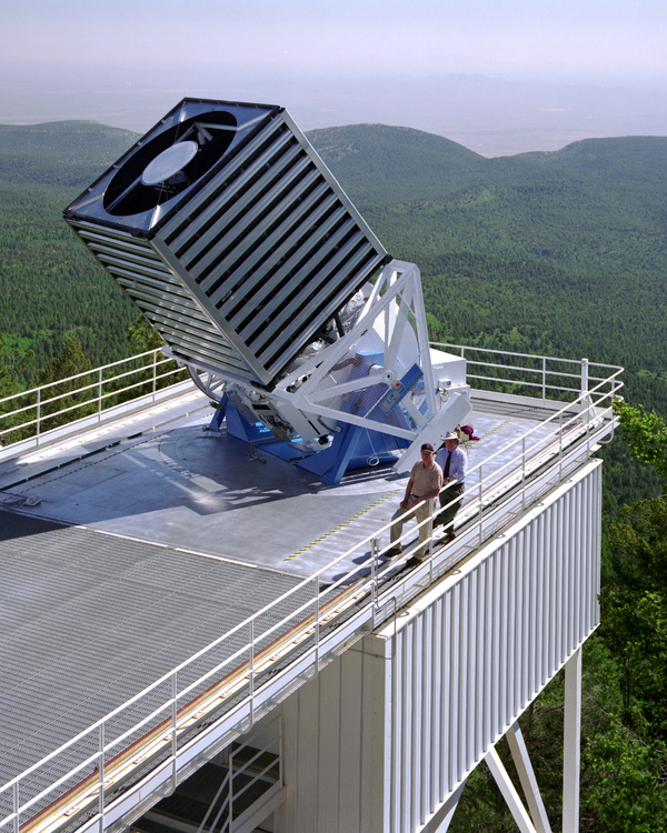
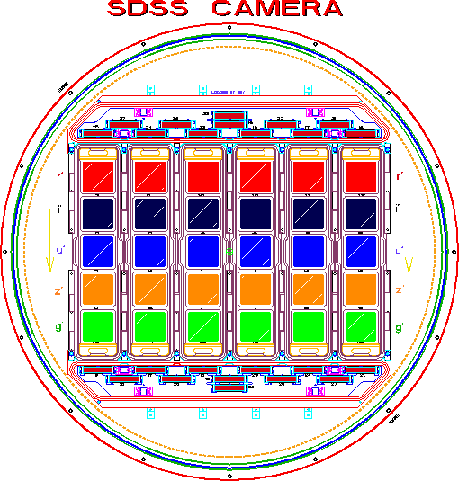
The main telescope has two main instruments; we'll ignore the spectrograph and concentrate on the mosaic imaging camera with 30 large CCDs, which acquires images in long strips through five differert filters nearly simultaneously:
For the most part, SDSS operations were designed to scan each region of the sky just once, in order to cover the maximum amount of space in the minimum amount of time. However, during the autumn seasons, when the main survey region wasn't easily scanned, the telescope was occasionally aimed at a section of the celestial equator. Over the years, this region was observed many times. During the period 2005 - 2007, the telescope scanned this equatorial stripe intensively in order to make a search for supernovae; you can go to the the SDSS Supernova Survey website for more details.
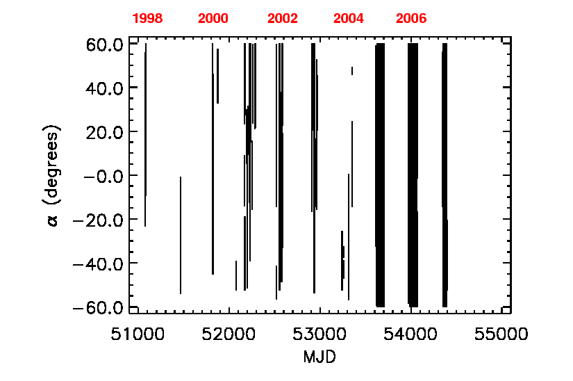
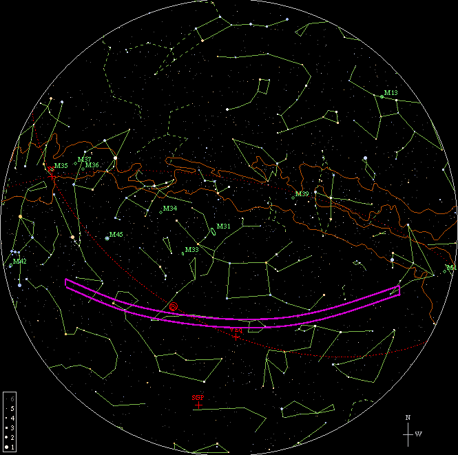
The region of interest lies along the celestial equator and stretches about 120 degrees from end to end.
The telescope scanned the sky at roughly the sidereal rate, yielding an exposure time of about 55 seconds in each of the five passbands, nearly simultaneously. So the observing cadence in each passband was pretty regular: once per night, every night or two for a few months, then no observations until the next autumn season. This is NOT an ideal way to plan measurements of most variable stars ... but, after all, the survey was designed to find supernova, which rise to prominence over a week or two and then fade over a month or two.
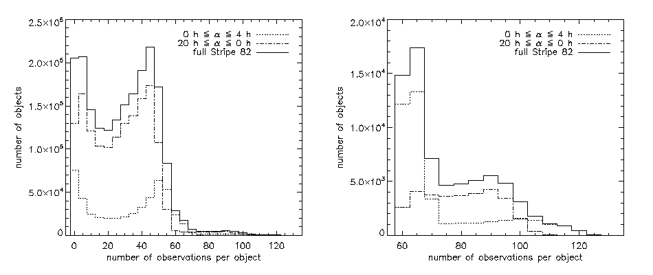
During the study period (1998 - 2007), most objects were detected about 30 times, but some were measured over 100 times.
The SDSS survey software took care of the basic steps:
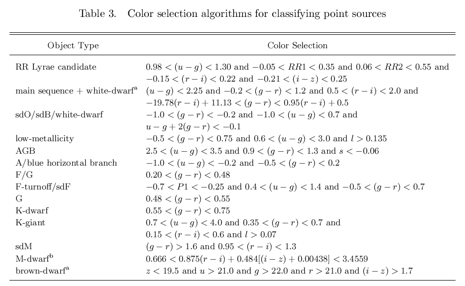
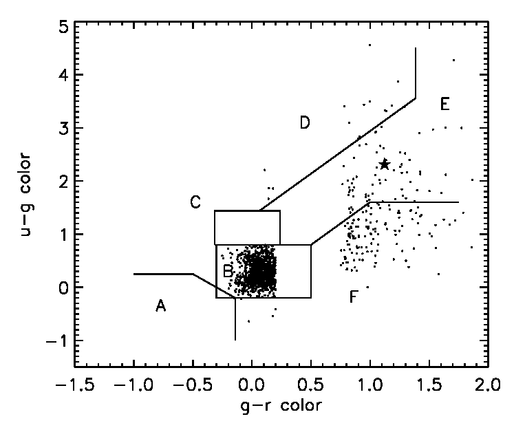
In addition, the many scientists involved in the SDSS determined many ways to use the colors of each object to determine its type. See, for example, Finlator et al., AJ 120, 2615 (2000).
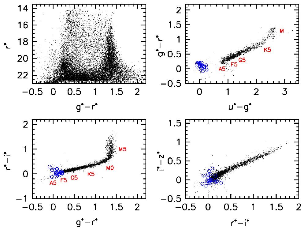
Figure 1 from Finlator et al. (2000)
We adopted rules like this to make rough classifications of point sources.
We were interested in stars (and quasars), so we discarded all the extended sources from the SDSS catalogs in this stripe. The result is a LARGE set of objects: over 57 million detections during the entire study period. It would have taken us too long to examine all of these objects by hand, so we created a pipeline to carry out a series of procedures on the entire set.
Let me mention briefly details about a few of these steps.
- Ensemble photometry
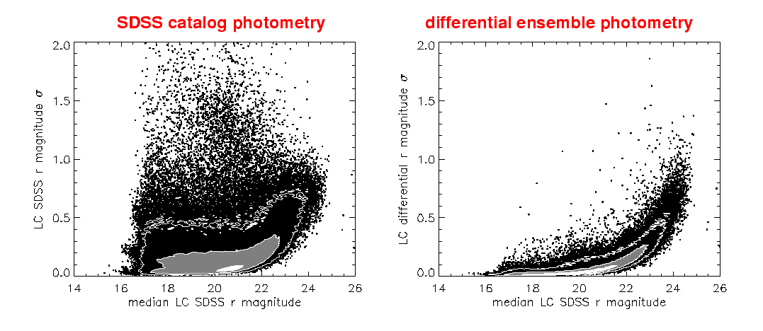
- Despite the care with which the original SDSS images were reduced and calibrated, there still remain small systematic differences in measurements made on different nights. In other words, on one night, ALL the stars in a small region appear to be a bit brighter than usual, and the next night, ALL the stars appear to be a bit fainter than usual.
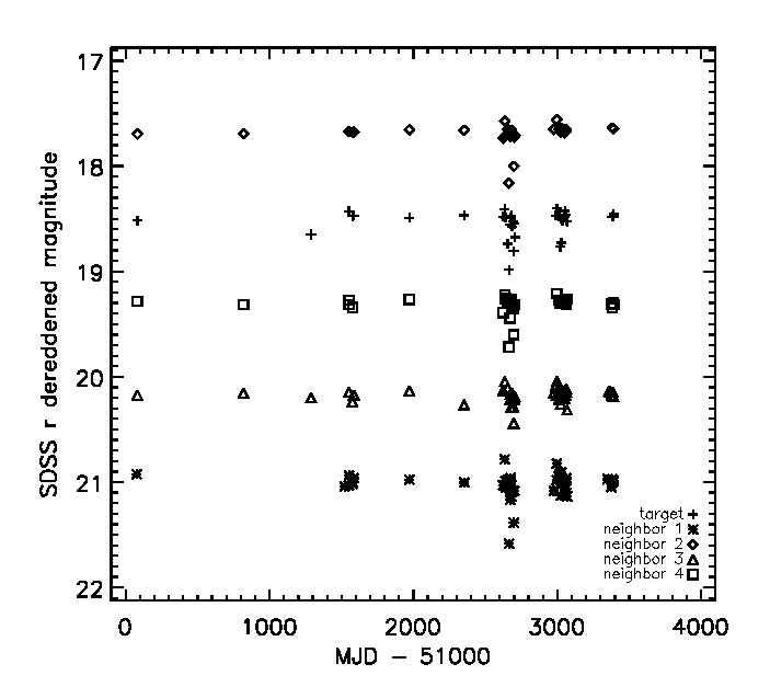
By looking at the behavior of all the sources in some region (an ensemble) over a long period of time, one can identify some of these systematic errors and remove them. The result will be a set of differential measurements which (usually) have signficantly smaller internal scatter.
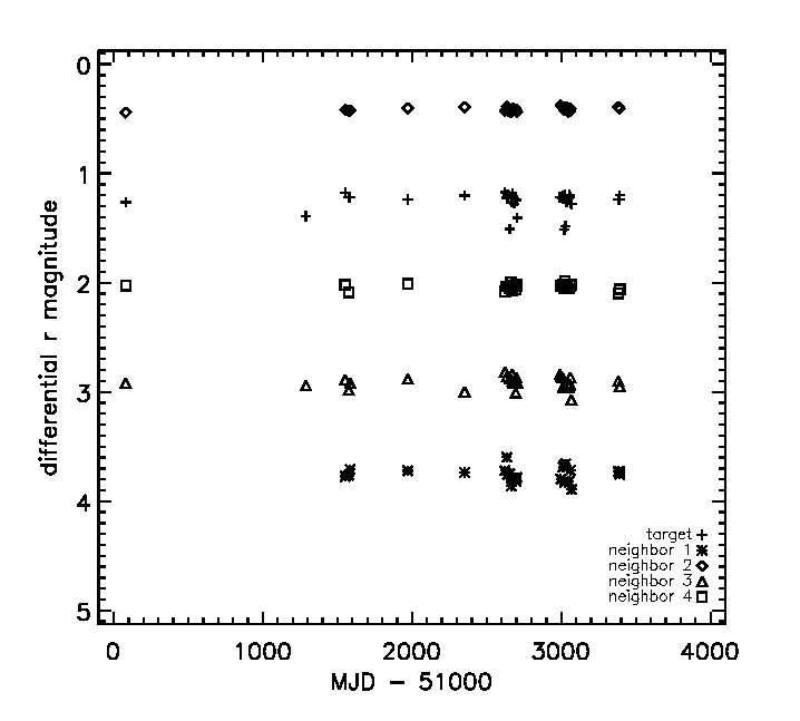
You can see the difference clearly if you plot the scatter from median magnitude against median magnitude:
- Detect variables using the Stetson index
- Objects with a larger-than-usual internal scatter are likely to be variable stars ... but there are still many false positives. A more sophisticated test for true variability makes the following assumption: a real variable star becomes brighter in ALL passbands as it rises, then fainter in ALL passbands as it fades. The Stetson variability index is a clever way to put this notion into a mathematical procedure. Consider two stars, each of which has mean magnitude 5.0. star A is a true variable, ranging from magnitude 4.5 to 5.5, while star B is actually constant, but has relatively large measurement errors. Suppose we measure each star in the V-band and I-band, and compute delta = (mag - mean_mag) for each measurement.
        date              Star A               Star B
                       V        I            V       I
      ---------------------------------------------------
       night 1        4.5      4.7          4.5     5.3
         delta       -0.5     -0.3         -0.5    +0.3

       night 2        4.7      4.8          5.2     5.2
         delta       -0.3     -0.2         +0.2    +0.2

       night 3        5.1      5.0          5.3     5.4
         delta       +0.1      0.0         +0.3    +0.4

       night 4        5.4      5.4          4.7     5.1
         delta       +0.4     +0.4         -0.3    +0.1
      ---------------------------------------------------
The basic idea behind the Stetson index is to multiply the delta values for the two bands each night, then add up the products.
      Star A

         index = (-0.5)*(-0.3) + (-0.3)*(-0.2) + (0.1)*(0.0) + (0.4)*(0.4)
               =    0.37

      Star B

         index = (-0.5)*(0.3)  + (0.3)*(0.2)   + (0.3)*(0.4) + (-0.3)*(0.1)
               =    0.0
Random variations will lead to equal numbers of products with positive and negative signs, whereas true variability will yield products with positive signs.
Out of roughly 360,000 objects with at least 10 epochs of measurements, about 8,500 are classified as "variable candidates" by our metrics.
- Check for periodic variations
- Some types of variable stars have periodic variations; most AGN and quasars do not. We checked each variable candidate for periodic variations using two techniques:
- "string-length" method ( Dworetsky 1983 )
- Phase-Dispersion Minimization (PDM) ( Lafler and Kinman 1965 )
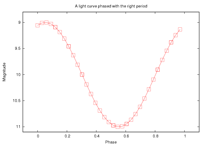
Neither method requires the variation to be sinusoidal. Each has the same basic idea: if you pick the right period, then some property of the light curve will be minimized. In the case of the "string method", the property is the length of an imaginary piece of string stretched from point to point along the phased light curve. If we pick a bad period, we'll need a long piece of string to connect the dots in order:

But if you pick the right period, the segments from one point to the next will be short:
This is just a little peek at a few results -- we are still working on it.
The fraction of point sources which appear to be variable is a strong function of color. In these color-color diagrams, the stellar locus runs from hot, blue stars (regions A and B in the lower-left) to cool, red stars (right-hand end of region E, F). Note the large fraction of objects with blue colors which are variable -- many of these turn out to be quasars.
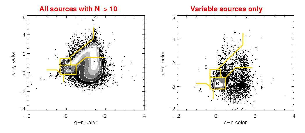
Objects which we identify as periodic variable stars appear, not surprisingly, along the main stellar locus. They are most common at the blue end.
If we select objects which are
we find quite a lot of objects which which are very likely to be quasars.
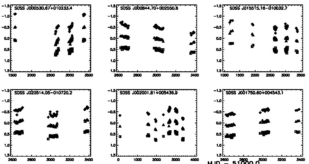
As is well known, many quasars vary over long timescales in the optical. Here are a small selection of objects which are marked as variable by our pipeline, and which appear in the catalog of SDSS quasars of Schneider et al., AJ, 134, 102 (2007) . Each object has three sets of symbols, showing its light curve in the SDSS g, r and i passbands.
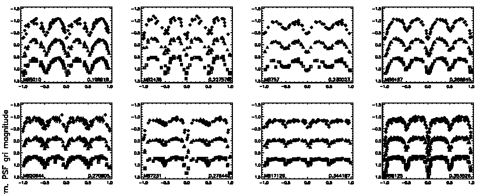
Our pipeline has identified a large sample of objects which are eclipsing binary stars.
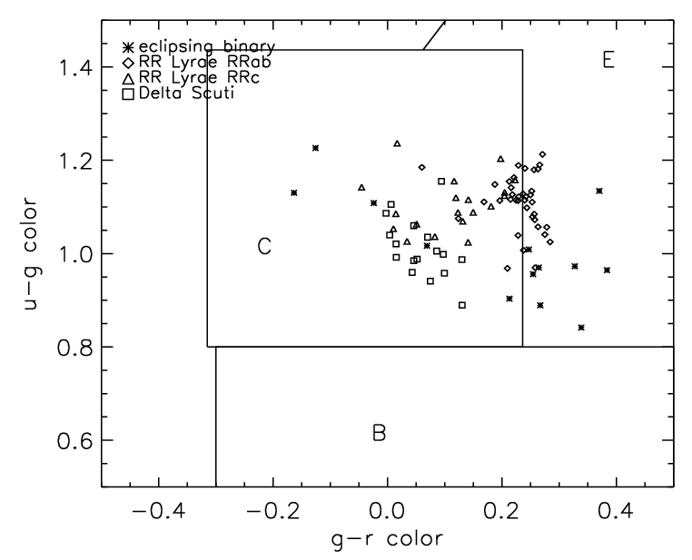
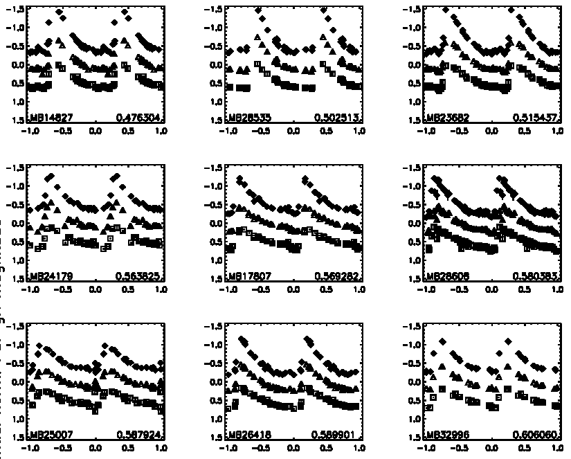
We can also select RR Lyrae stars easily by finding periodic variable stars with light curves described by certain combinations of Fourier components. Here are some pretty RRab stars.
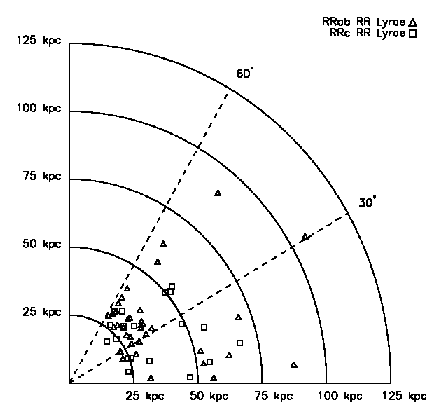
Since we know the absolute magnitudes of RR Lyrae stars, we can calculate their distances with some accuracy. This sample isn't large enough to break any new ground, of course, but it's fun to look at where these stars fall within the Milky Way.
Copyright © Michael Richmond.
This work is licensed under a Creative Commons License.