 Copyright © Michael Richmond.
This work is licensed under a Creative Commons License.
Copyright © Michael Richmond.
This work is licensed under a Creative Commons License.
We'll begin by discussing galaxies in a general way today, focusing on the several systems astronomers use to classify galaxies. I'll mention some of the most common terms used to describe galaxies, and we'll spend a bit of time discussing the ways that one can describe quantitatively the distribution of light observed in galaxies.
But before we can get to any of that, it's necessary to introduce the notion of surface brightness, since this will be an important factor in many studies of galaxies.
What exactly does the term "surface brightness" mean, anyway? And why does it only appear in discussions of galaxies, but not stars? Let's take a closer look.
Ordinary "brightness" refers to the amount of light our eyes or instruments collect from some particular source. If we detect more photons from source A than from source B, we say that source A is brighter than source B. Simple enough.
When we observe stars with ordinary telescopes, we see tiny points of light. The apparent "size" of each star doesn't really have anything to do with the physical extent of the star; instead, it's just an artifact of the instrument we use, the wavelength at which we observe, and, most important for ground-based observations in the optical, the atmosphere through which the light has passed. The Point-Spread Function (PSF) created by the atmosphere and the optical system sets the area over which each star's light is spread. For ordinary ground-based optical telescopes, the PSF is typically a few arcseconds in diameter.
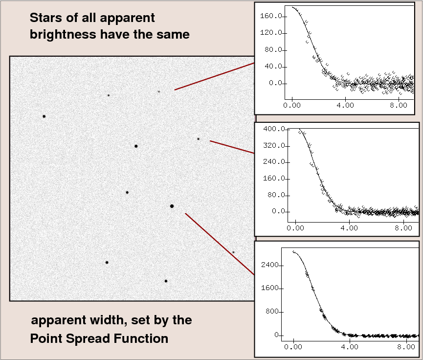
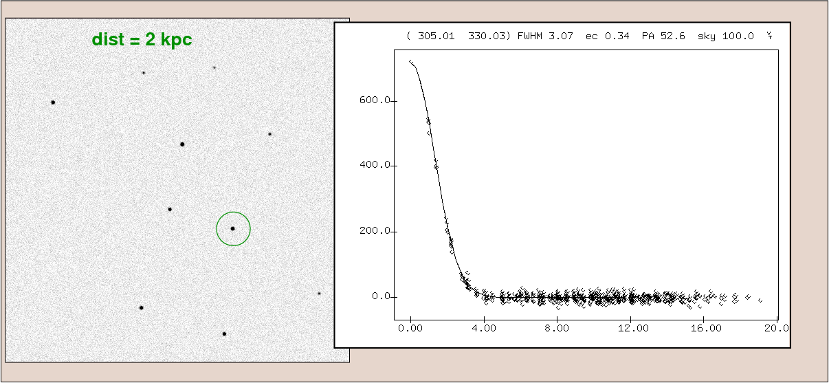
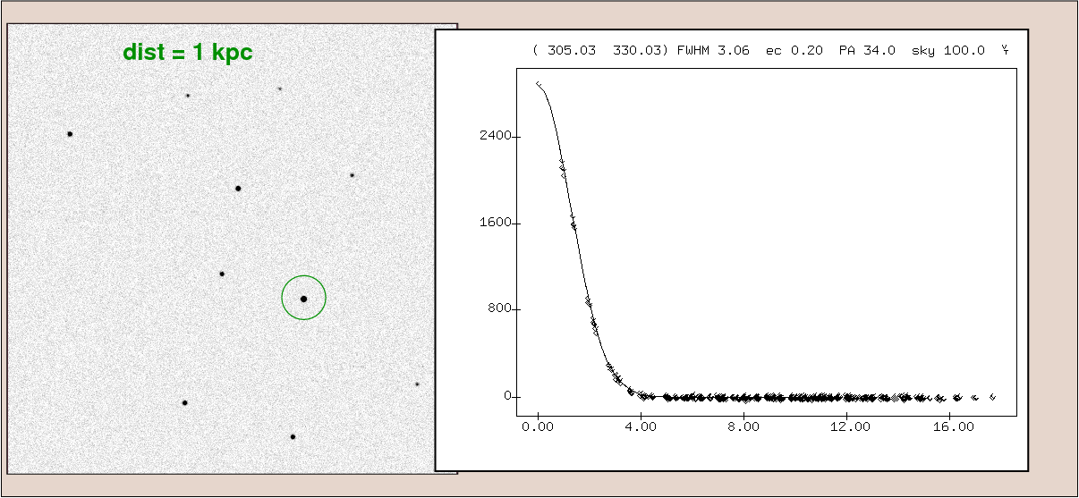
So, what would happen to the appearance of a star if we moved it to different distances away from the Earth? Suppose we observe a star initially at a distance of 1 kpc. Our instruments measure a peak of about 2800 counts per pixel at the center of the PSF.

If the star is moved twice as far away, to a distance of 2 kpc, then intensity of the light from the star falls by a factor of 22 = 4, due to the inverse square law. The apparent size of the star, however, doesn't change at all: it is still set by the PSF. The result is that the intensity at the center of the star's image falls by a factor of 4.
If we continue move the star farther away, to 4 kpc and 8 kpc, we'll continue to see the star grow fainter and fainter, until it finally disappears into the noise.
Now, we can define surface brightness as some quantity which describes the amount of energy received from some angular area on the sky per unit time. The unit of angular area is usually chosen to be square arcseconds.
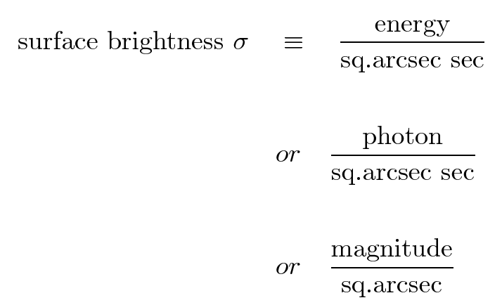
In practice, one can measure surface brightness by drawing a box of some known angular area in an image, adding up all the light detected within the box, and dividing by the area of the box. For example, we might use a box of height 3 arcseconds and width 3 arcseconds, making an area of 9 square arcseconds.
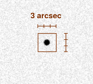
If we measure all the light falling into this box from a single star, we can compute the surface brightness in the following manner:
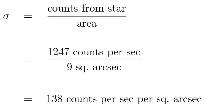
In most published work, the instrumental units of "counts per second" would be replaced by calibrated units such as "magnitudes"; in order to do the conversion, one must know how many counts per second would be gathered by the same instrument from some star of known brightness.
Now, if we were to move the star twice as far away, our instruments would register a source with the same apparent size and shape (that of the PSF), but only 1/4 the brightness. We would therefore find that the surface brightness of the star would decrease as its distance from us increased, via the usual inverse square law.
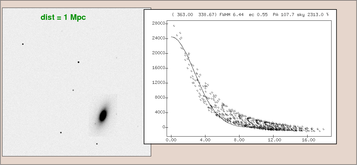
On the other hand, suppose that we take images of a galaxy which is 1 Mpc away. The light of the galaxy is spread out over a large angular area, much larger than the PSF. The image below contains about 28,000 counts per pixel near the center of the galaxy.

If we were to move the galaxy twice as far away, to a distance of 2 Mpc, the apparent size of the galaxy would decrease .... but look at the central intensity.
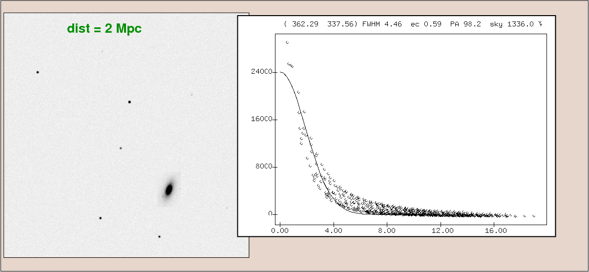
The number of counts in the central region of the galaxy remains close to its initial value. Why is that?
That means that the surface brightness, measured in counts per second per pixel, or magnitudes per square arcsecond, will remain the same as the distance to the galaxy doubles.
As long as the galaxy is signficantly larger than the PSF, the surface brightness of the galaxy will remain constant. Note that the total apparent brightness DOES decrease: even though "magnitudes per square arcsecond" is the same, the galaxy covers fewer square arcseconds.
What's so great about surface brightness, anyway? It's important because many of the methods we use to survey the sky aren't really limited by the apparent brightness of objects as much as they are limited by the surface brightness.
For example, below is a picture showing a portion of the sky in the constellation of Andromeda. You can see plenty of stars, but can you find a galaxy?
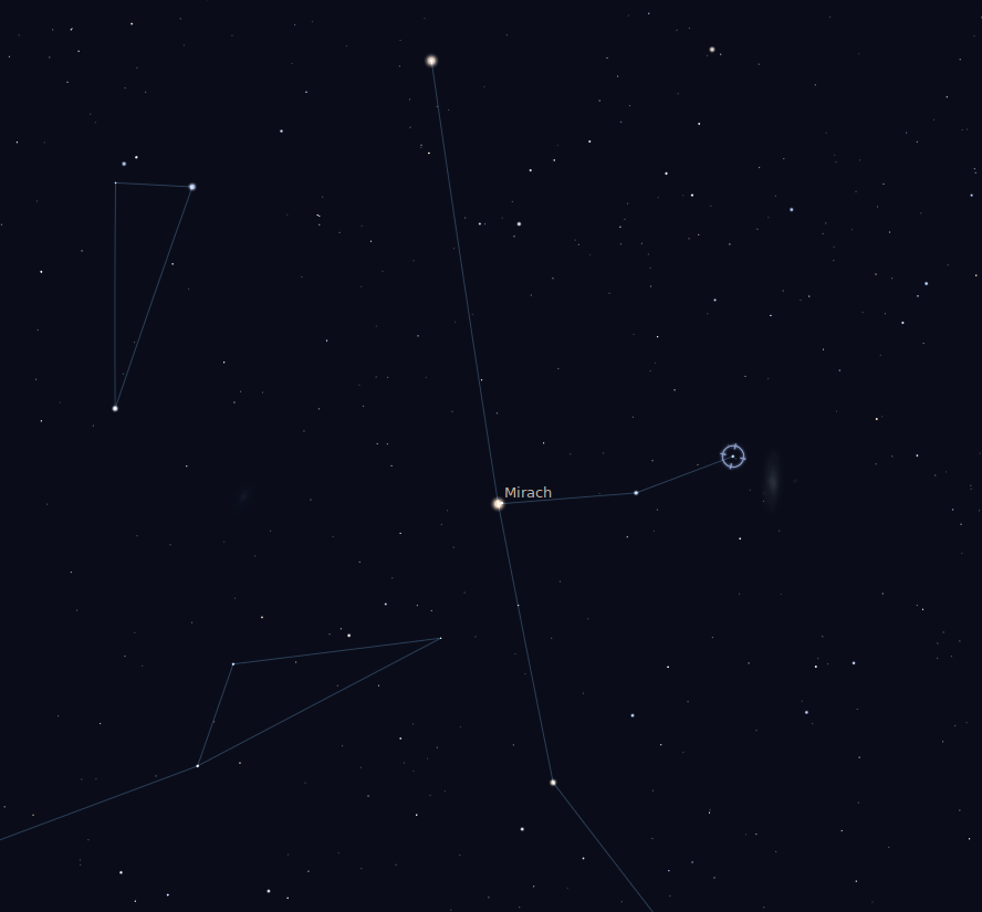
Of course you can -- there's M31.
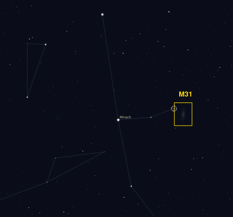
But do you see the other galaxy, too? I'll give you some help --- see these two stars? They are about the same total magnitude as the other galaxy: Star A = HIP 9570 has V = 5.50, while star B = HIP 8433 is V = 5.75,
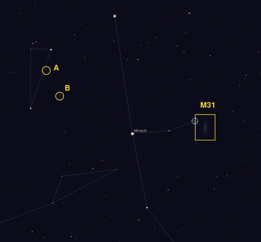
The other galaxy is M33, which has integrated magnitude of V = 5.7. But its light is spread out over a much larger area, so it doesn't stick out from the background.
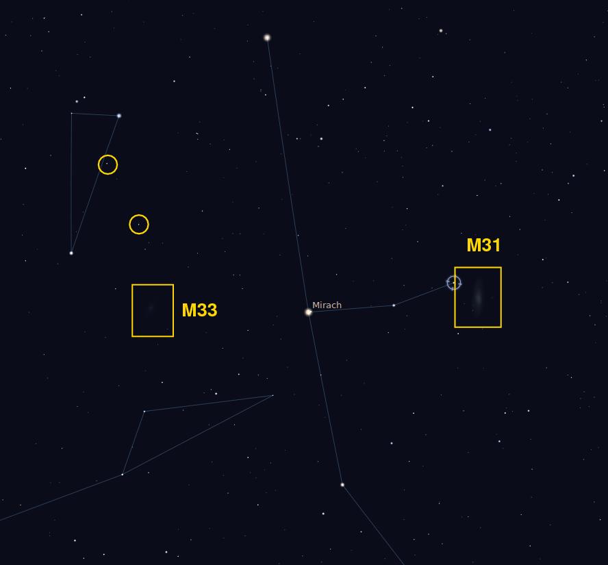
Notice the diffuse nature of the light from this galaxy -- even the nucleus lacks any great concentration.
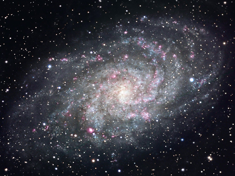
Image courtesy of
Giovanni Benintende
When you think of galaxy catalogs, what letters come to your mind?
The first two were complied on the basis of visual measurements -- yes, eyeballs looking through telescope eyepieces. The latter two were made by people sitting in warm rooms indoors (that's the good news), painstakingly sliding magnifying glasses across big photographic plates (that's the bad news). Consider these extracts from the introduction to the UGC:
In order to make the Catalogue as complete as possible and to avoid large inhomogeneities in the measurements, the Sky Survey prints have been searched through three separate times. The Catalogue is based mainiy on the last two surveys. Each survey continued for approximately one year.The galaxies have always been searched for on the blue prints. The prints have been surveyed through an S.0.C. "Visolett" magnifier with a magnification of X 1.6 and a diameter of 3.5 cm. The procedure was to survey first the right-hand half of the prints from the bottom upwards, and the lens was moved in "sweeps", with so much overlap that every object was expected to enter in the field of view at least three times. The same procedure was then applied to the left-hand part of the print, with sufficient overlap between the two halves. Every galaxy expected to be close to 1'.0 or larger was measured with the Leitz magnifier. At least two separate settings were made for each diameter, with the measuring scale in opposite orientations.
Objects with very low surface brightness are less likely to be detected in surveys of this nature. Therefore, much of our understanding of galaxies has been tilted towards those galaxies which have higher surface brightness. What does "higher surface brightness" mean? In this case, it's pretty close to "a high density of stars"; after all, more stars per cubic kpc of space means more stars per square arcsecond projected onto the sky, which means more photons coming from that square arcsecond.
Take a look at this region of the Sloan Digital Sky Survey. Where's the biggest galaxy?
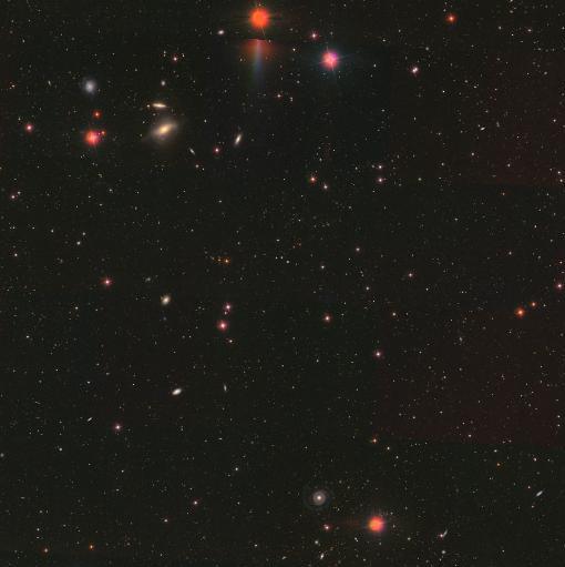
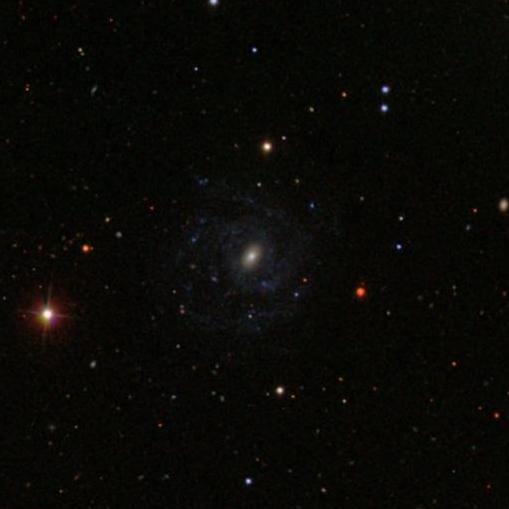
Dod you select the face-on spiral near the bottom of the picture? UGC 6614 covers such a large region on the sky that its arms tend to fade into the background. It's actually quite impressive, once you notice it.
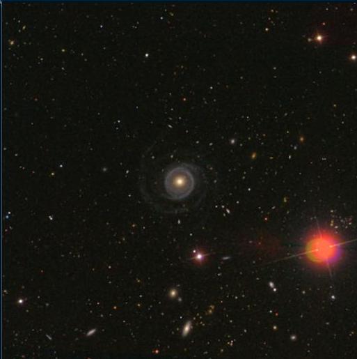
Try another one: where's the face-on spiral in this picture?
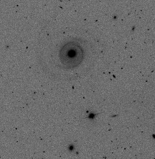
Look to the lower-left of the saturated pinkish stars near the top of the picture. You should find NGC 9024, another galaxy with low surface brightness.

The bottom line is that our most commonly used galaxy catalogs are biased in favor of galaxies with high surface brightness; and since much of current extragalactic science is based in part on those catalogs, it's very likely that some of our knowledge of galaxies may suffer from that bias.
Galaxies are complex structures, consisting as they do of billions of individual stars, giant clouds of gas and dust and pervasive yet invisible amounts of dark matter. It should be no surprise that different astronomers have chosen to classify them in different ways.
In the image below, the central galaxy NGC 5982 is an elliptical, flanked above (NGC 5981) and below (NGC 5985) by spirals.
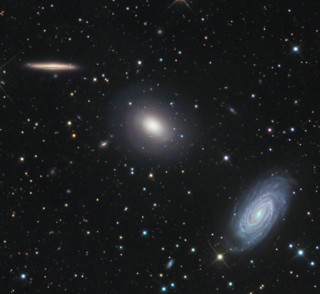
Image by Giovanni Benintende ,
thanks to
Astronomy Picture of the Day.
In his book The Realm of the Nebulae, Edwin Hubble organized galaxies into a sequence which splits spirals into normal and barred families, yielding the familiar "tuning fork diagram".
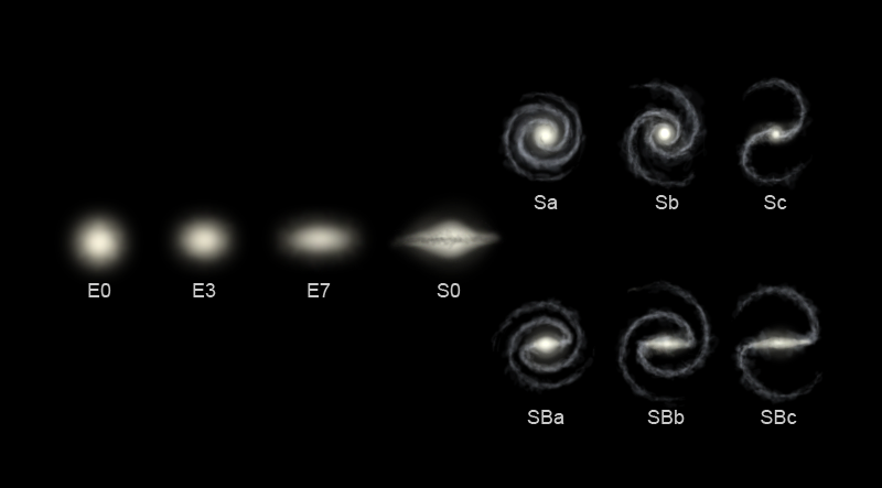
Image courtesy of
The Las Cumbres Observatory
The criteria used to place galaxies on this diagram are
Ellipticals are given a designation of the letter "E" plus a digit, where the digit represents the ellipticity of the galaxy's outer isophote, multiplied by 10:

The designations given to spiral galaxies are less easy to quantify; they rely on visual inspection of the galaxy and a long experience of classifying galaxies. The general idea is to assign a letter between a and d to each spiral galaxy, with Sa meaning "large bulge, tightly wound continuous arms" and "Sd" meaning "small bulge, loosely wound flocculent arms". Perhaps the best explanation of the procedure can be found in The Hubble Atlas of Galaxies .
The diagram shown above suggests that the difference between, say, an SBb and SBc galaxy should be easy to see. In real life, galaxies tend to be messy, as the diagram below indicates; it shows real images of galaxies.

Image courtesy of
Los Cumbres Observatory.
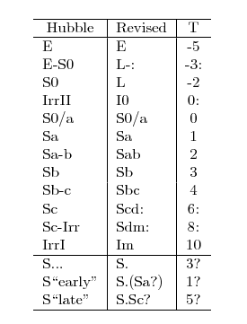
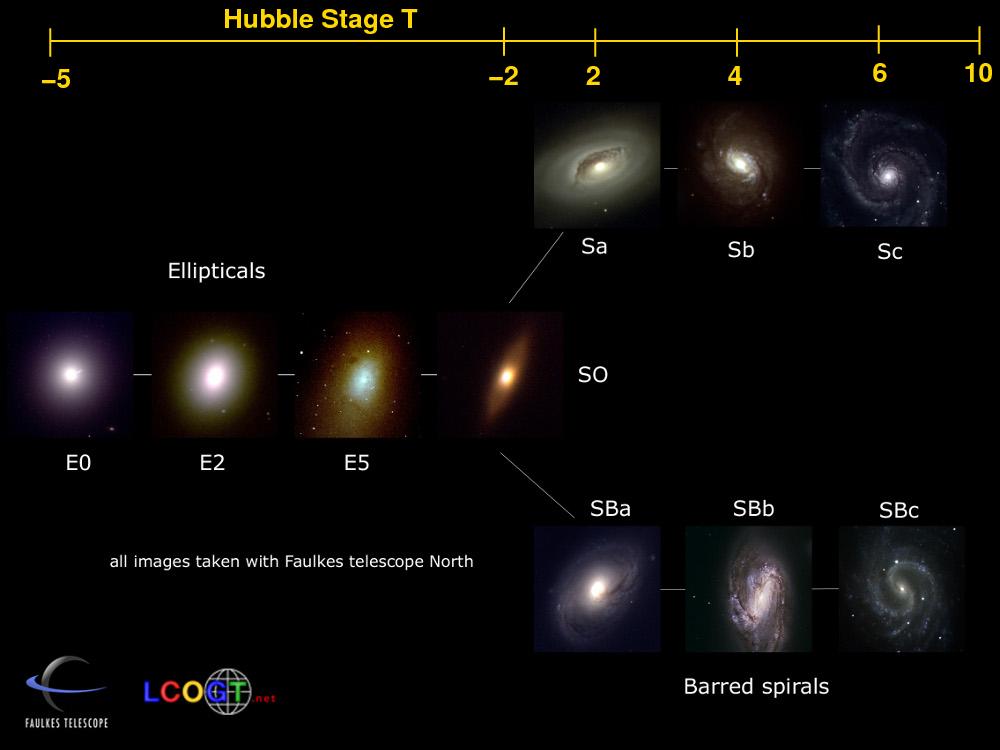
In 1981, the Second Reference Catalog of Bright Galaxies (RC2) by deVaucouleurs et al. provided a means to put all galaxies onto a semi-quantitative scale. The "Hubble Stage" parameter T is an integer value ranging from -5 (for ellipticals) to +10 (for irregulars).
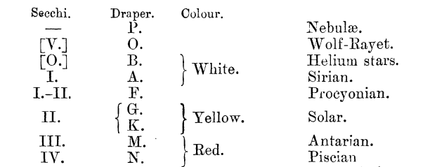
when applied to stars
Taken from
The Observatory, vol 38, p 379 (1915).
Some scientists believed that this same sequence, from hot to cold, described the evolution of individual stars over time. In this way, the term "early" came to be applied to the hot O and B stars, and "late" to the cool K and M stars.
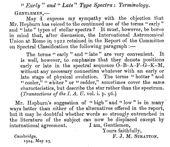
By the nineteen-twenties, this view had fallen out of favor, due to increases in the understanding of stellar structure. Nonetheless, the words "early" and "late" continued to be applied to stars following the earlier convention. This annoyed some people
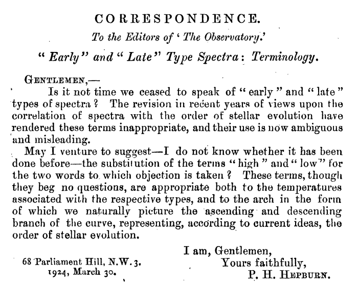
but failed to sway the IAU, as this correspondence shows.
when applied to galaxies
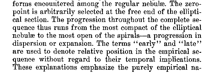

As a result, the terms "early" and "late" have stuck to galaxies, with the sense that "early-type" galaxies are centrally concentrated and redder, while "late-type" galaxies are more diffuse and bluer.
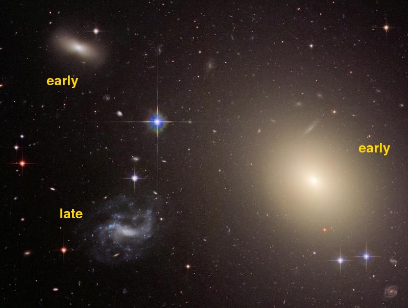
Note the internal inconsistency: early-type galaxies are dominated by late-type stars, and late-type galaxies by early-type stars. Sigh.
One choice for a numerical measure of concentration is based on ratios of the radii which contain specific fractions of the total light of a galaxy. Let us define
Now, these values will certainly change if we move a particular galaxy closer to or farther from the Earth; but the ratios of these quantities might not. One can use the concentration indices
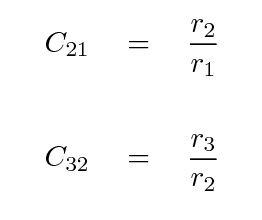
to describe the degree to which light in a galaxy is collected near the center. Large ratios means that the light is highly concentrated, while small ratios mean that the light is diffuse.
Early work showed hints that high concentrations were found among elliptical galaxies, and lower concentrations among spirals, but the evidence wasn't all that persuasive. This figure comes from an article in 1973.

More recent work (published in 2001) based on digital images shows that the correlation between the concentration of light and morphology really is pretty good. Alas, this particular paper -- and much of the recent work -- adopts a new definition of "concentration index" which is roughly the inverse of the previous one, so in the figure below, small values of C mean the light is highly concentrated.
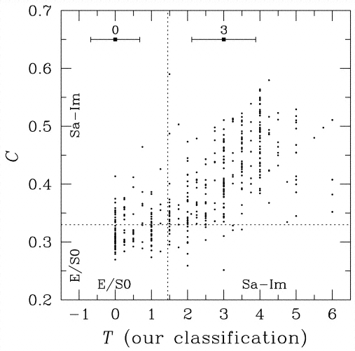
Figure 10 from
Shimasaku et al., AJ 122, 1238 (2001)
Below you can see the radial profile of an ordinary elliptical galaxy on the left, and a cD on the right.
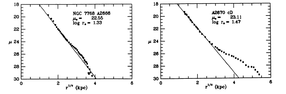
Figure 1 from
Schombert, ApJS 60, 603 (1986)
Compare this spectrum of NGC 6090 (from the SDSS)

to this spectrum of the ordinary galaxy PGC 57421 which sits next to it in the sky

Figure taken from
Prieto et al. MNRAS 402, 724 (2010)
We'll talk more about AGN later.
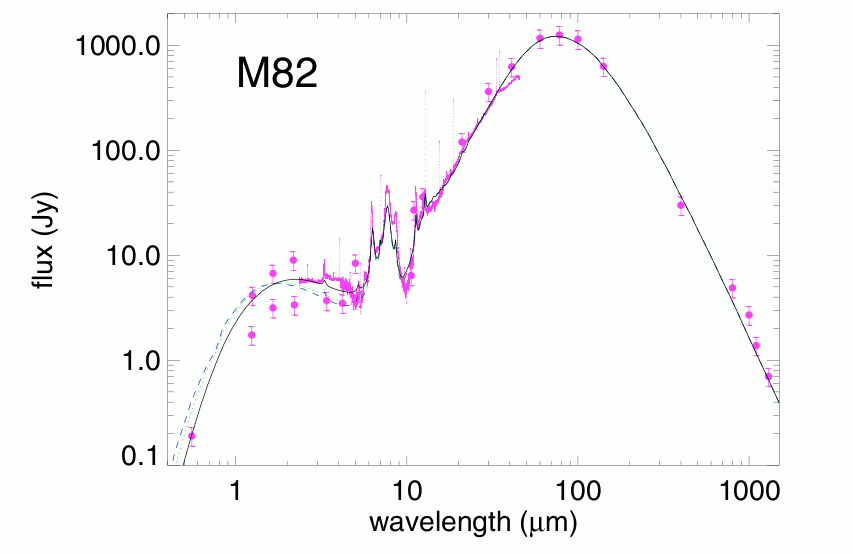
Figure taken from
Siebenmorgen and Krügel, A&A 461, 445 (2007)
We know the properties of millions of galaxies, which makes it possible to study the distribution of many factors over the entire population. Perhaps the most basic question one can ask is "Are there more high-luminosity or low-luminosity galaxies?" A more nuanced version of this question is "Exactly how common are galaxies of different luminosities?" The answer to this question can be expressed with a luminosity function.
We begin by picking some volume of space -- let's call it V cubic Mpc. We then survey the volume to find and measure all the galaxies within it. Let L be some luminosity, which might range from, say, 106 solar luminosities for a tiny dwarf galaxy to perhaps 1011 solar luminosities for the most powerful quasars. If we pick some small range in luminosity, from L to L + dL, we can count the number of galaxies N which fall within that range. The galaxy luminosity function is then defined by

Of course, we could also measure the luminosity in terms of absolute magnitude, in which case we have a slightly different flavor of the luminosity function:
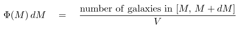
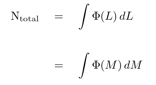
Either way, if we integrate the luminosity function, we should end up with the total number of galaxies inside our volume.
Back in 1976, Paul Schechter devised a simple analytic function which seemed to describe the luminosity function of galaxies quite well.
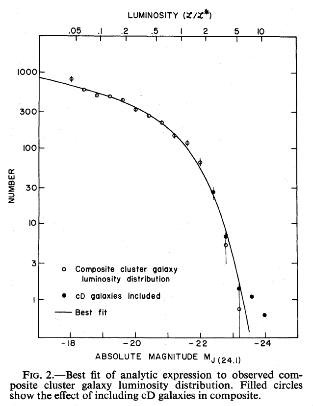
The function looks like this:
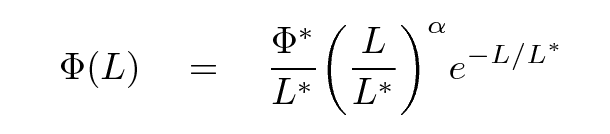
The three parameters are
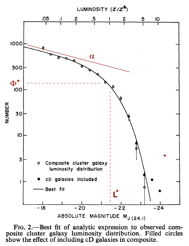
Astronomers like the Schechter function: it's relatively simple, does a decent job of fitting the observations, and it is easy to deal with analytically. However, there are dangers to using it. First, note that the density of galaxies appears to grow without bound as one looks at fainter and fainter luminosities; if one were to extrapolate to very low luminosities, one might predict an infinite number of galaxies, or an infinite amount of light. Neither is correct (obviously).
One must also keep in mind that these fits are based on observations which had various sorts of bias. Very luminous galaxies, for example, are rare; we don't see any galaxies with M = -24 near the Local Group, so we must rely on samples covering huge volumes and large distances to count them. But at those large distances, we can't detect at all the very common, low-luminosity galaxies which we can and do find in the Local Group. In order to make a graph like the one above, one must mix and match results from different surveys, each with its own set of biases. It's a complicated business.
There's a nice little warning by Anthony Smith about these dangers. The diagram below shows some observations from the UKIRT Infrared Deep Sky Survey and a range of Schechter function fits to the measurements. The different colors show what happens if one uses only a subsample of all the galaxies to determine the parameters of the Schechter function.

Copyright © Michael Richmond.
This work is licensed under a Creative Commons License.