 Copyright © Michael Richmond.
This work is licensed under a Creative Commons License.
Copyright © Michael Richmond.
This work is licensed under a Creative Commons License.
Suppose we observe some galaxy in the sky.
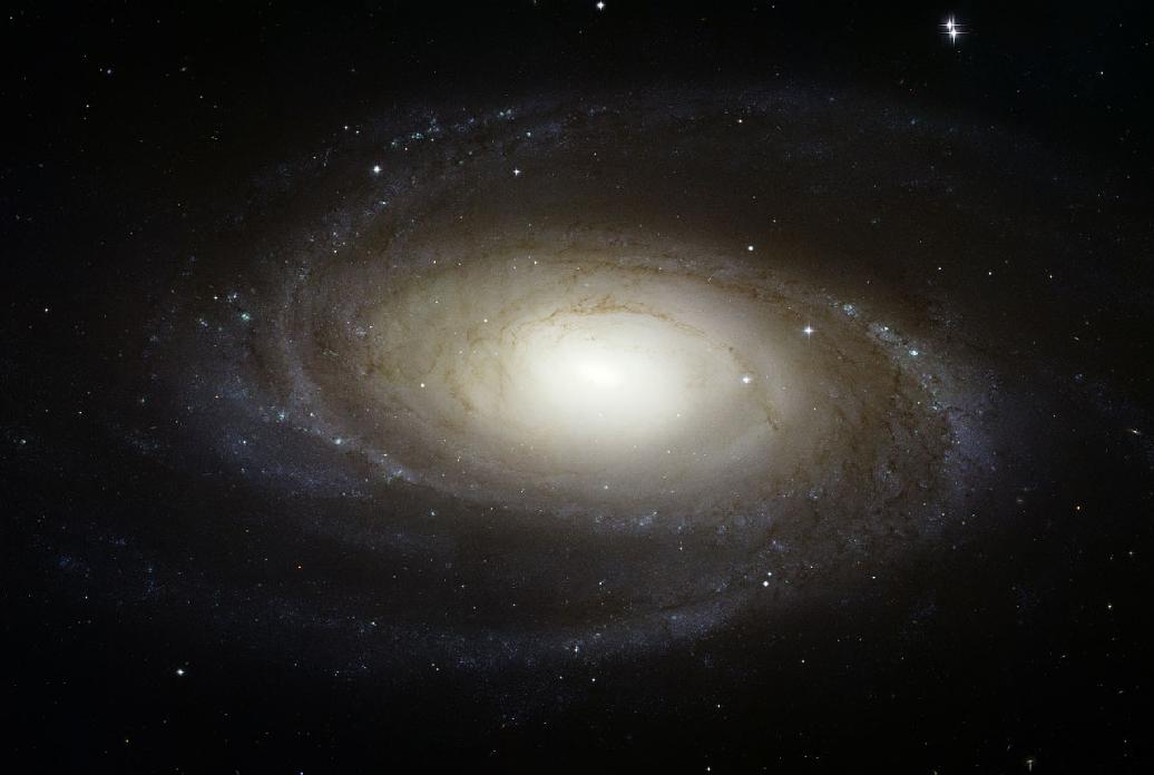
Let's measure the intensity of light as a function of radius, averaging over all the pixels in circular annuli.
The result will be a set of pairs of measurements: radius r and intensity of light at that radius, I(r). We can express it in a table ...
| radius (pixels) | intensity (counts per pixel) |
| 1 | 1209.3 |
| 2 | 1087.5 |
| 3 | 853.2 |
| 4 | 522.7 |
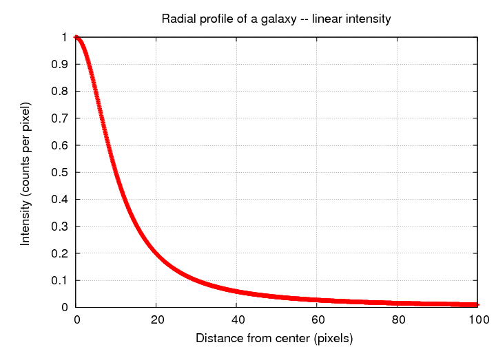
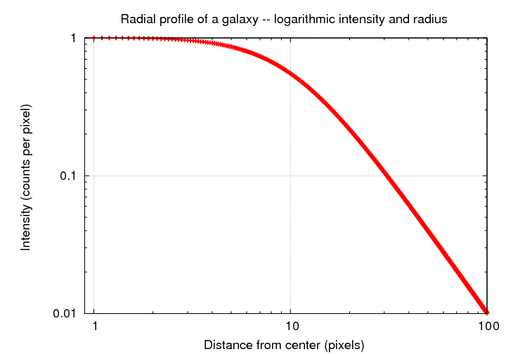
We can also display this information in the form of a graph. Now, there are many possibilities for making a graph. We can use linear units for both intensity and distance from the center:
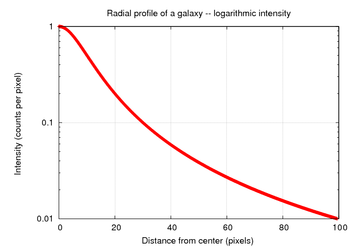
... or we may choose to use logarithmic units for intensity -- if we used magnitudes, for example -- which can yield a very different profile shape:
... or we may choose to use logarithmic units for BOTH intensity and for radius:
Galaxies are three-dimension entities, but we only get to examine them from one point of view. Therefore, when we take an image of galaxy, and measure the amount of light coming from some small region an angular distance α from the center,
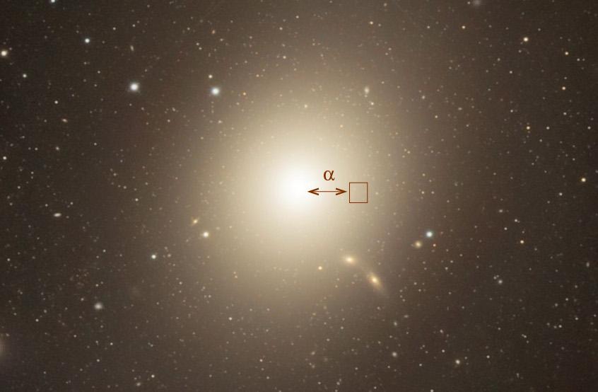
Image courtesy of
Robert Gendler
via
Astronomy Picture of the Day
we are NOT just measuring the light coming from one tiny little chunk of the galaxy;
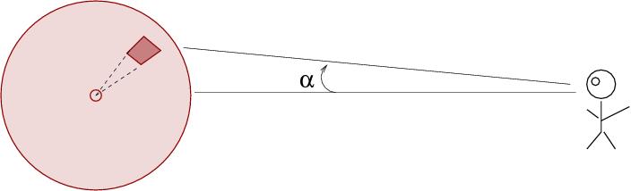
instead, we are measuring the sum of all the light contributed by a long, thin pencil of material from the galaxy.
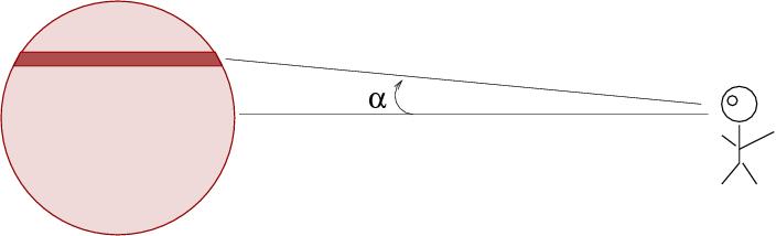
If one were strict, one might speak of a distribution of light within a small chunk of the galaxy located a radial distance r from the center, at a position given by angles θ and φ; and then one might speak of a DIFFERENT distribution of light, obtained by integrating the first distribution over a line of sight through the galaxy.
Astronomers are, for the most part, not so strict. Most of the time, a paper discussing I(r) means "the surface brightness of light measured at a projected distance r from the center of the galaxy."
Still, it's good to keep this in mind. Theorists who build 3-D models of the stellar distribution within a galaxy must project their models onto a 2-D surface in order to compare the models to our observations.
In practice, we can't measure the radial profile of a galaxy out to arbitrarily large radii because, at some point, the light from the galaxy disappears into the noise of the background sky. Many of the big galaxy surveys were based on a few sets of photographic plates, such as the POSS I and POSS II . The uniform properties of these plates allowed astronomers to choose a particular surface brightness which was close to the apparent limit of galaxies on most of the plates. This limit of about m(B) = 26.5 mag/sq. arcsec was used to measure the apparent size and shape and brightness of galaxies in some catalogs; the radius at which the surface brightness falls to this level is called the "Holmberg radius", and the contour defined by this surface brightness the "Holmberg isophote."
If you find measured parameters for a galaxy, such as its diameter, but no description of the method used to make the measurement, it might very well be based on this Holmberg isophote.
One common quantity used to describe galaxies is the effective radius or re, which is defined as the radius which contains half the total light of the galaxy. So, if we were to plot the cumulative sum of light integrated from center outwards as a function of radius,
the radius at which the sum reaches half of its eventual value is the effective radius.
Galaxies are scattered throughout the universe at a vast range of distances from us. In order to compare galaxies to each other fairly, we must find some description which doesn't depend on distance -- which would yield the same value if a galaxy were suddenly to move to twice its current distance.
In 1976, Vahe Petrosian described one approach which removes distance from the equation. His approach is somewhat complicated, so let's take it one step at a time.
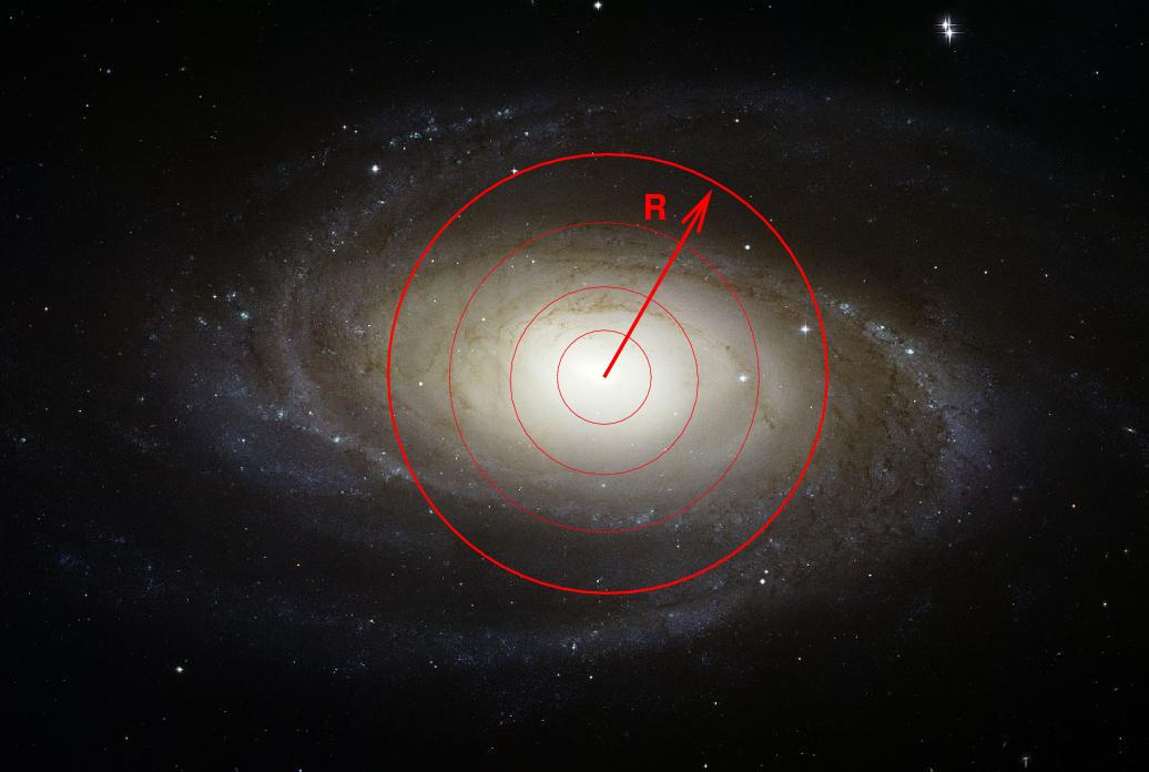
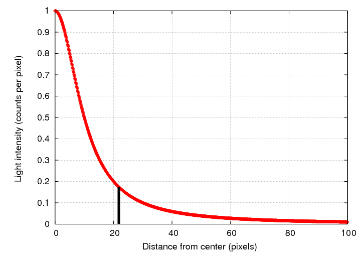
Start with the radial profile of light in some galaxy. Pick some radius R -- we'll try 22 pixels. In the example below, the intensity at R appears to be about 0.18 counts per pixel.
Now, integrate all the light from the center out to R.
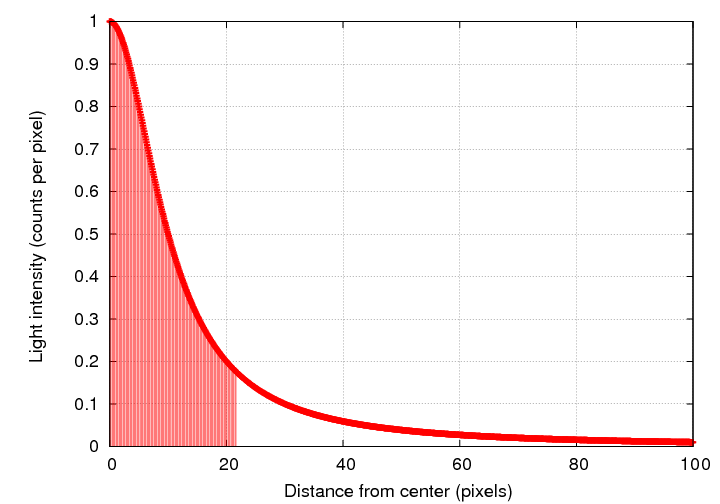
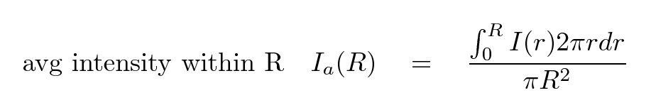
Compute the average intensity of light within the radius R; it's just the integral of light over area within R, divided by the area of a circle with radius R.
We can plot this average intensity as a function of radius, of course. At our chosen distance R, the integrated average intensity Ia(R) is about 0.38 counts per pixel.
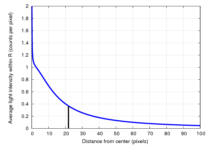
So, to recap, in our example, at the radius R = 22 pixels,
These two measures aren't the same. But, if we had chosen a somewhat larger radius, then the average intensity within that radius would have been lower; and, if we had chosen just right, we might have found a location at which I(R) = Ia(R). This is the idea behind the Petrosian radius RP.
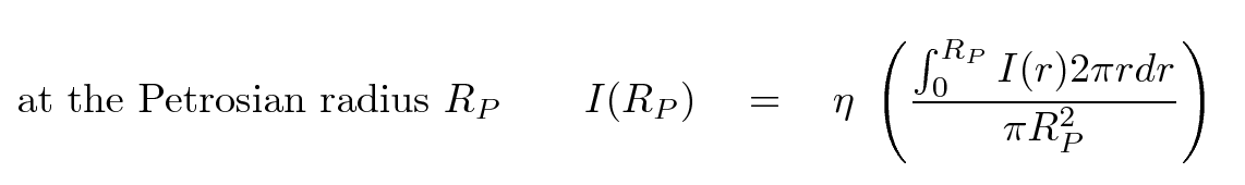
where η is some constant of order unity. In an ideal world, we might choose η = 1 for simplicity; but in the real world, it turns out that the radius at which the local intensity is equal to the average interior intensity turns out to be pretty small; small enough that the presence of seeing can modify it significantly. By choosing a radius farther from the center, where the local intensity is just, say, 0.5 or 0.3 times the average interior intensity, we can make a better measurement. In Shimasaku et al. (2001) , for example, the authors choose η = 0.2. The SDSS photometric pipeline followed their lead and adopted the same value η = 0.2.
The important point is that, regardless of the exact choice of η, the Petrosian radius RP is independent of distance. It is also insensitive to reddening by dust in the foreground.
Once we have this special radius, we can use it to measure other quantities which will similarly be independent of a galaxy's distance.
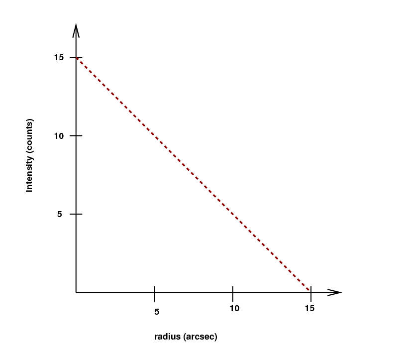
Consider a galaxy which has the radial profile of intensity shown below.
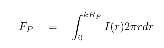
Why don't we just use k = 1? For the same reason that we don't choose η = 1 -- practical considerations. Typically, the surface brightness of a galaxy is still pretty high at the Petrosian radius, so we can improve our signal-to-noise ratio by including more of the galaxy's light than falls within RP itself. The SDSS, guided by Yasuda et al. 2001 and Shimasaku et al. (2001) , chose to make k = 2.
Once again, remember that there is a good reason to make all these complicated definitions: by measuring galaxies in this fashion, we can compare nearby objects to distant ones in a proper manner.
Copyright © Michael Richmond.
This work is licensed under a Creative Commons License.