 Copyright © Michael Richmond.
This work is licensed under a Creative Commons License.
Copyright © Michael Richmond.
This work is licensed under a Creative Commons License.
The idea for this test is pretty simple: pick objects which are identical in size S and observe them at a range of distances. The angular diameter distance DA will be related to the apparent angular size of the objects θ.
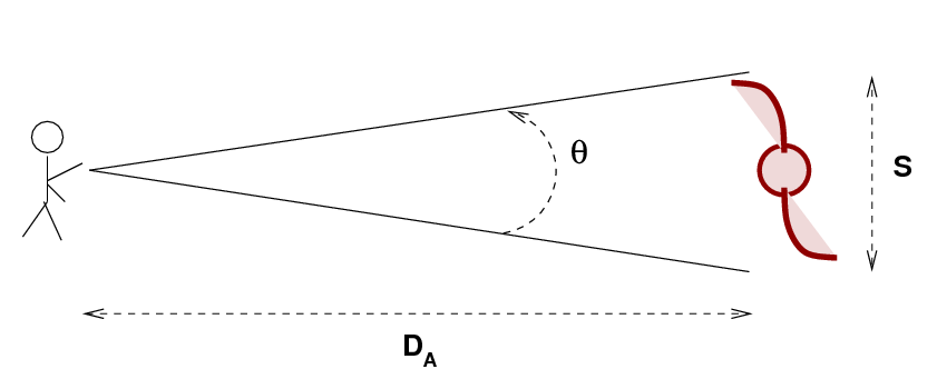
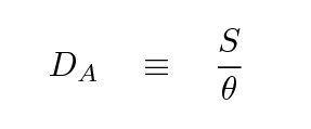
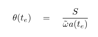
If we use radians as the units for the apparent angular diameter, and if the object is at a large distance, then
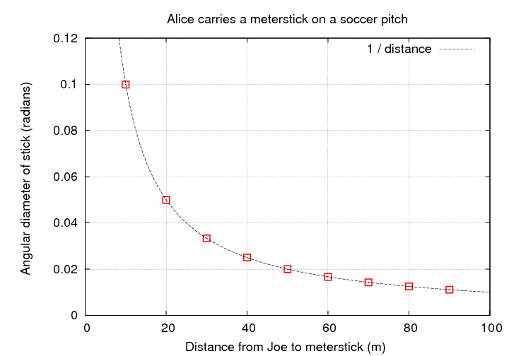
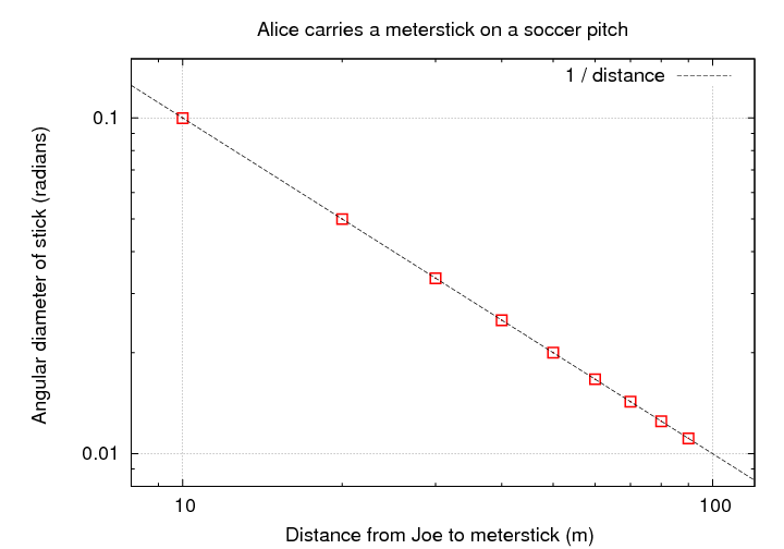
Now, in an ordinary Euclidean space, like a nice flat soccer pitch, the relationship between apparent angular size and distance is simple. If Joe stands at one end of the field while Alice carries a meterstick to the other end of the field, and Joe makes a series of measurements of the apparent angular size as a function of distance,
  Q:  What relationship between apparent angular
      size and distance will Joe find?
Well, this relationship is simple enough in Euclidean space. But what will happen if we use sources at cosmological distances in an expanding universe? In this case, the angular size depends on the diameter of the source and on the proper distance between the source and observer at the time te when the light from the source was emitted.
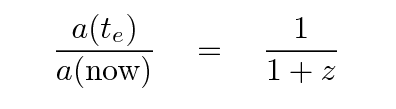
In order to compare theory to observations more easily, we should convert from time of emission te to redshift z. The denominator of the expression above has two pieces: the comoving coordinate ω and the scale factor a. Let's consider them separately.
The scale factor at the time when light was emitted (long ago) is related to the scale factor when the light is absorbed by our telescopes (now) in a simple manner:
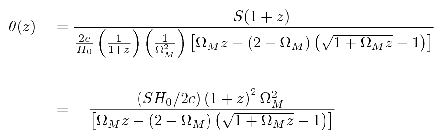
So the angular size as a function of redshift becomes
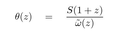
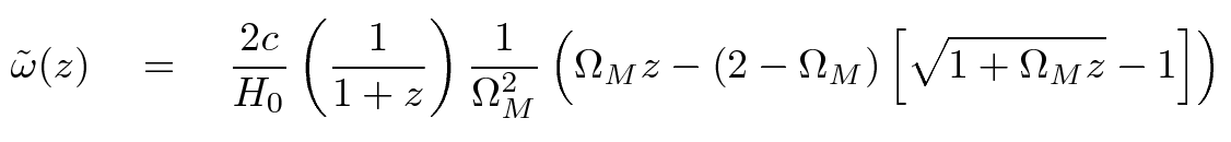
The comoving coordinate at the time the light was emitted is a more complicated function of redshift. If we continue to assume that the cosmological constant ΩΛ is zero, then
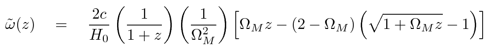
Thus, we find that the angular size as a function of redshift is pretty complicated.
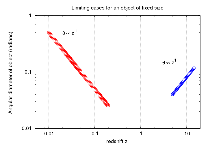
Let's look at the limiting cases: what happens at small redshifts, when z ~ 0? What happens at large redshifts, when z >> 1?
  Q:  Simplify the expression for θ as a
      function of redshift for z << 1.


  Q:  Simplify the expression for θ as a
      function of redshift for z >> 1.
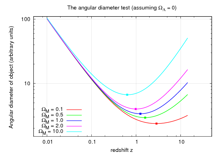
Evidently, the angular size of objects must reach a minimum value and then start to INCREASE with distance! One can show that if ΩM = 1, then the location of this minimum angular size is at z = 1.25. It increases for smaller values of ΩM and decreases for larger values.
Now, what can we use as our "standard yardsticks" in the sky? Ideally, we would find a type of object which
That last requirement is the tough one. Giant elliptical galaxies, for example, satisfy the first two requirements, but how exactly would one define the size of an object which gradually fades away? Moreover, why should all giant elliptical galaxies be identical in size?
In the nineteen-sixties and nineteen-seventies, astronomers turned to radio galaxies as a possibility. Some of the brightest radio sources in the sky were associated with giant galaxies (and giant ellipticals, in particular).
The observations of radio sources weren't quite as clean as one might have hoped. Consider this comparison of angular size and redshift from 1978:
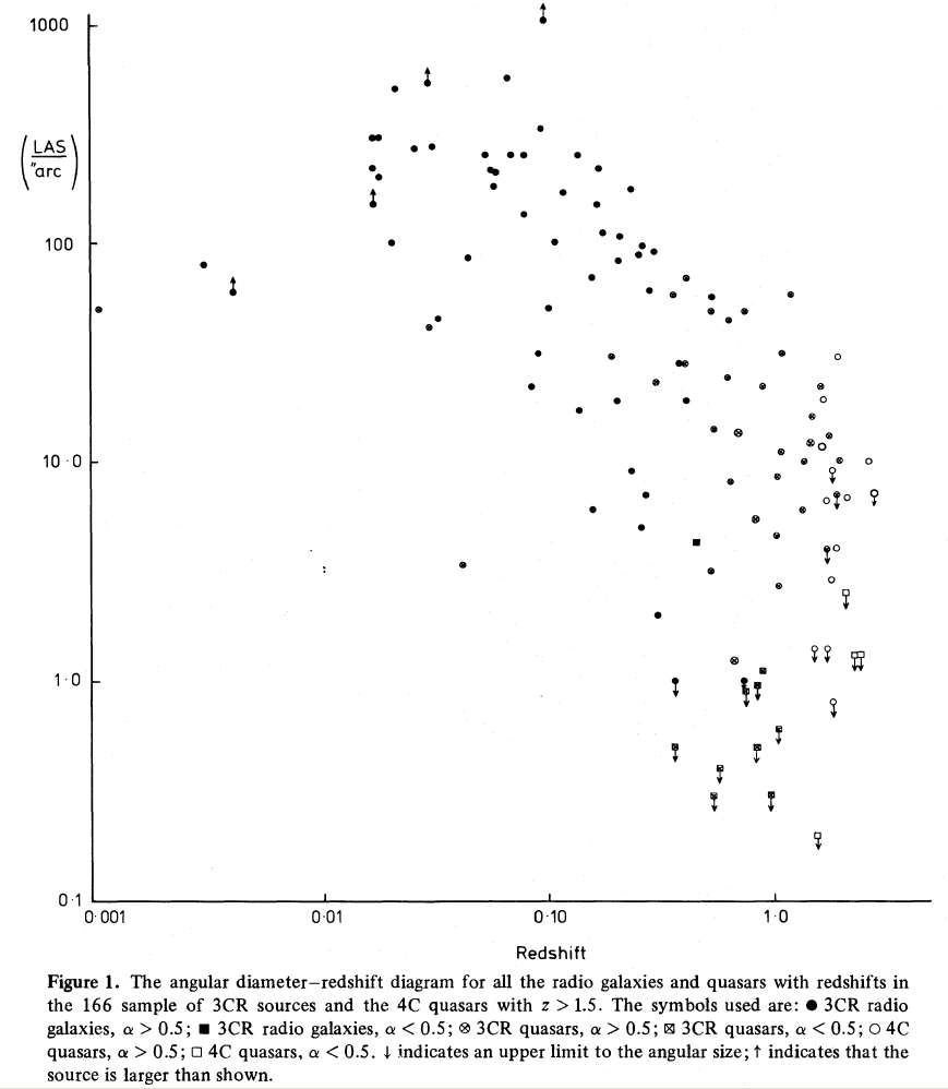
Figure taken from
Hooley, Longair and Riley, MNRAS 182, 127 (1978)
Here's a subset of the same dataset, plotted together with two cosmological predictions.
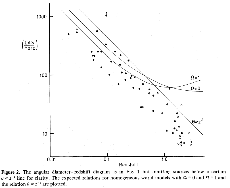
Figure taken from
Hooley, Longair and Riley, MNRAS 182, 127 (1978)
As Hooley, Longair and Riley stated in their abstract,
This is indeed the Achille's heel of the angular-diameter test: are radio sources really constant in size at different redshifts? Or, if they do shrink (or grow) at high redshift, just how quickly does their size change? We must also keep in mind that BIG sources are very likely to be MORE LUMINOUS than small ones; therefore, at high redshift, there is likely to be a strong bias against detecting the smaller, less luminous sources.
The angular diameter test, alas, seems to depend more upon our assumptions about the properties of radio sources than it does on the cosmological parameters.
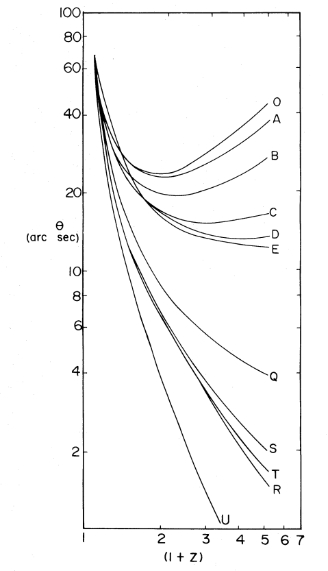
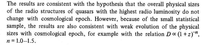
Figure taken from
Okoye and Onuora, ApJ 260, 370 (1982)
In the figure to the left, there are predictions for the angular diameter test for a large range of possibilities.
![]()
Nine years later, Onuora (1991) was still struggling with ambiguities in the data. The graph at left shows galaxies as circular symbols, and quasars as crosses. The author concluded that orientation and evolution made it difficult to draw any conclusions.
![]()
The angular diameter test has fallen out of favor in the past decade or two. My guess is that astronomers have realized that the "standard yardsticks" of the skies -- radio sources -- suffer from too many complicating factors to be effective distance indicators. After all, now that astronomers can use radio interferometers to resolve these sources and map their properties clearly, we know that the radio emission from these distant galaxies is not coming from the same regions as the optical light. In many cases, the radio emission turns out to be due to a compact core surrounded by two lobes. A relativistic jet carries material from a central AGN outward until it smashes into the intergalactic medium, where it excavates giant "bubbles" of low density material. The three sources shown below were all included in the studies above.
Figure taken from
The NRAO Image Gallery
Figure taken from
The NRAO Image Gallery
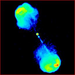
Image taken from
The Atlas of DRAGNs
It is no surprise now that radio galaxies are not "standard yardsticks."
One of the other classic tests uses "standard candles" rather than "standard yardsticks." The idea is to measure the apparent brightness of a set of objects which emit the same luminosity, but are at a range of distances. The relationship between apparent magnitude and redshift depends on the luminosity distance as a function of redshift. If we can measure that relationship precisely, we can extract the cosmological parameters from the equation for luminosity distance.
In the previous lecture , we derived expressions for the luminosity distance. It depends in part on the comoving coordinate as a function of redshift,
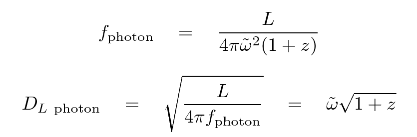
and in part on the manner in which one chooses to measure the brightness of a source; if one uses a photon-counting device,
or, if one uses an energy-measuring device,
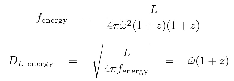
For the remainder of this discussion, we will adopt the photon-counting luminosity distance. Many of the conclusions we reach would be the same if we were to adopt the energy-measuring version, although the detailed numbers would be slightly different.
Let's begin with a review of Mr. Hubble's work. If we can measure properties of the local universe alone -- as was the case in the 1930s and 1940s -- then what can we learn from the magnitude-redshift relationship? Well, to find out, we can look at how luminosity distance depends on the value of two parameters in particular.
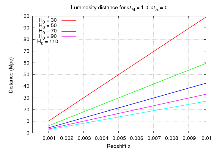
  Q:  If we look at the nearby universe, which of the
      cosmological parameters can we measure?


  Q:  Use the graph below to estimate the value
      of that parameter.
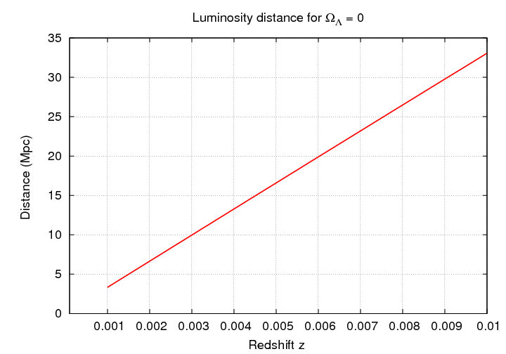
Notice the quantities plotted on the vertical axis of this graph: distance, in units of Mpc. In most cases, astronomers measure the APPARENT magnitude of some type of object -- supernovae or galaxies.
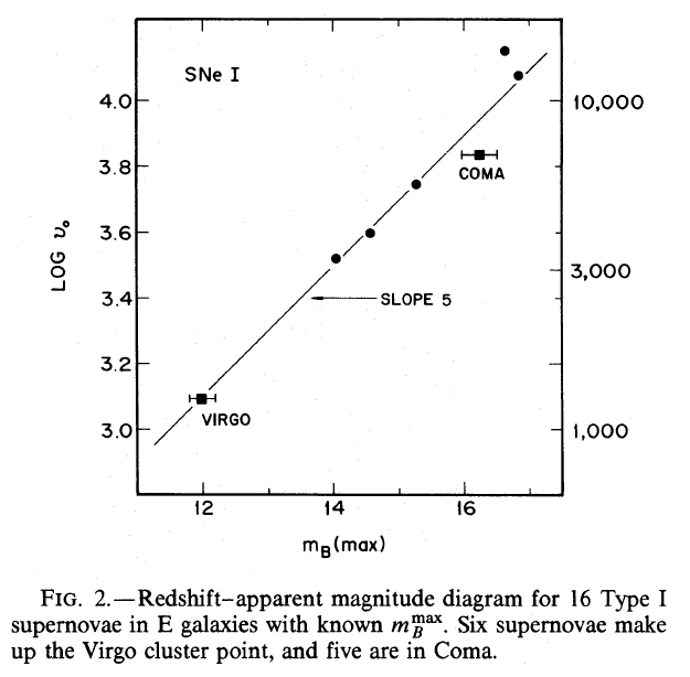
Figure taken from
Sandage and Tamman, ApJ 256, 339 (1982)
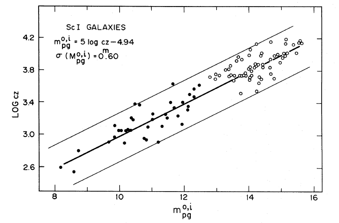
Figure taken from
Sandage and Tamman, ApJ 197, 265 (1975)
In order to compute the distance, we need to know the ABSOLUTE magnitude of that class of object. This is an important point:
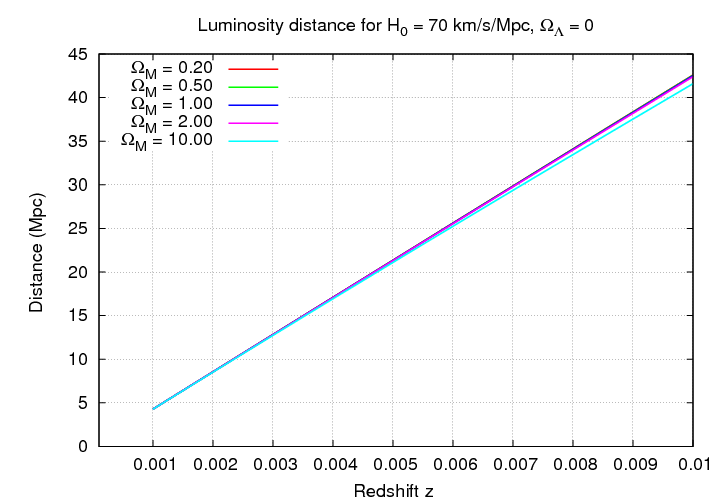
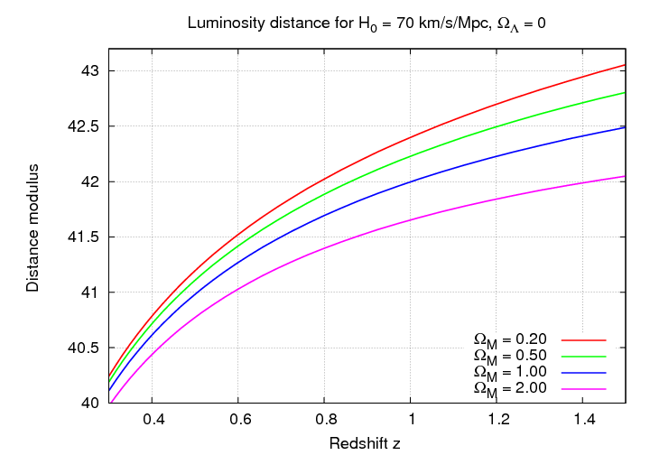
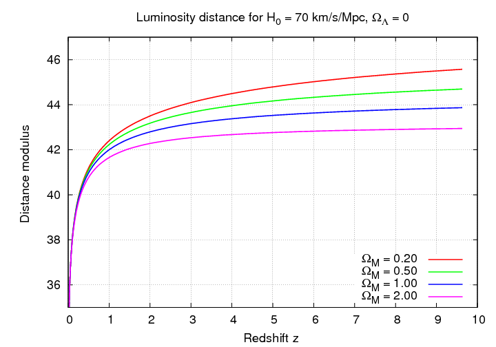
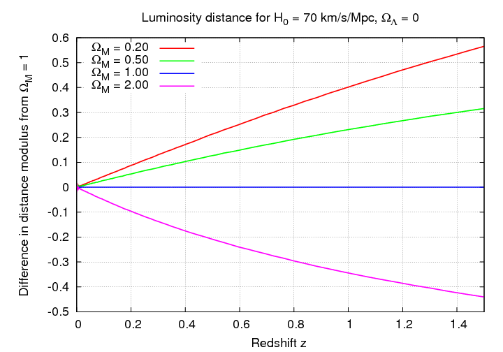
If we are interested in the ΩM parameter, then we must look much farther afield. The difference between the apparent magnitudes of some standard candle in different cosmologies only becomes significant once we extend our observations to redshifts greater than z > 0.5, or, better yet, z > 1.
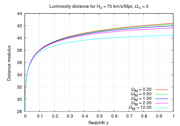
  Q:  Which value of ΩM produces
      the largest distance modulus?


      Explain.
Let's look at little more closely at some of the models.
  Q:  If one can measure objects out to z = 0.5,
      how 'standard' must the standard candles be
      to distinguish models with ΩM = 0.5
      from models with ΩM = 1.0?


  Q:  If one can measure objects out to z = 1.0,
      how 'standard' must the standard candles be
      to distinguish models with ΩM = 0.5
      from models with ΩM = 1.0?


  Q:  If one wishes to measure ΩM
      to a precision of 10 percent, and one can detect
      objects out to z = 1.0, how 'standard' must
      the standard candles be?
Notice that the effect of the Hubble constant at these large scales is pretty simple: without changing the SHAPE of the relationship, it just shifts the distance values
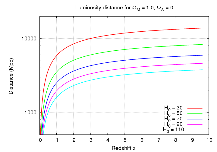
or the distance modulus values.
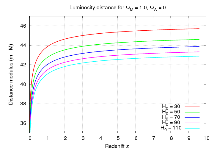
For example, compare the graph above to the graph below.
This is actually a very useful feature of the redshift-magnitude relationship in this regime. Even if we don't know the ABSOLUTE value of some standard candle, we can still use it to investigate the cosmological parameters. As long as all instances of some particular type of object have exactly the same luminosity/absolute magnitude, the SHAPE of the redshift-magnitude graph will reveal the underlying parameters.
Let's pick our standard candle: Type Ia supernovae. There is good evidence that these objects do have the same absolute magnitude, with the caveats
In the late nineteen-nineties, two groups of astronomers searched for high-redshift supernovae. They had to find the supernovae, measure the light curves well enough to determine peak magnitudes and the shape (in order to correct for shape-dependent effects), and -- this is the hard part -- acquire a spectrum to verify that the event really was a Type Ia and to measure its redshift.
Q: Why was getting a spectrum "the hard part"?
Let's look at their results, which were published in 1998 and 1999.
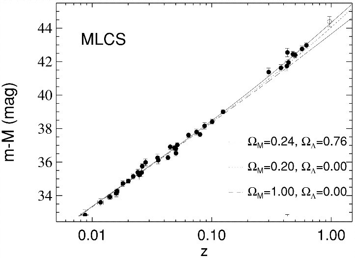
Figure taken from
Riess et al., ApJ 116, 1009 (1998)

Figure taken from
Perlmutter et al., ApJ 517, 565 (1999)
Now, as you can see, all the interesting action is stuffed into the upper-right corner of these graphs. It might be easier to answer some of these questions if we made a slightly different graph. Let's change the vertical axis so that we plot the difference between the distance modulus for some particular model and the distance modulus for some benchmark model; say, ΩM = 1.0.
So, again, here are the results from the supernova studies.
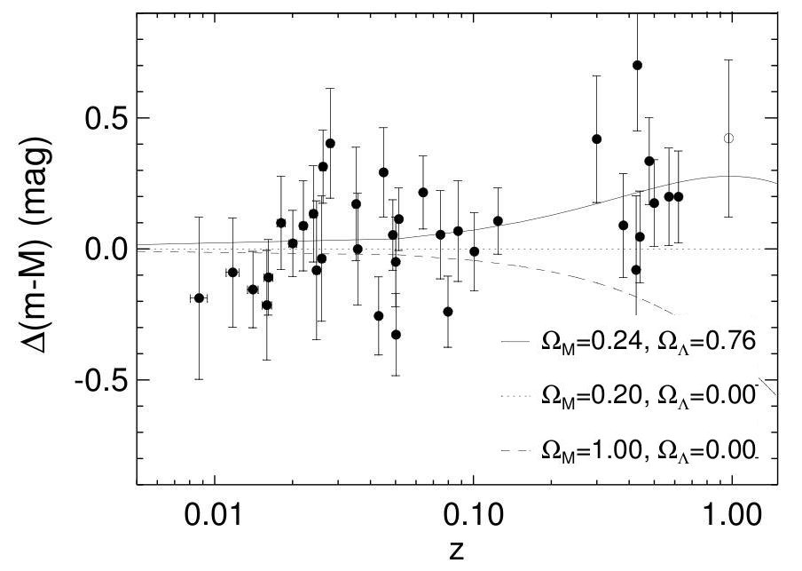
Figure taken from
Riess et al., ApJ 116, 1009 (1998)
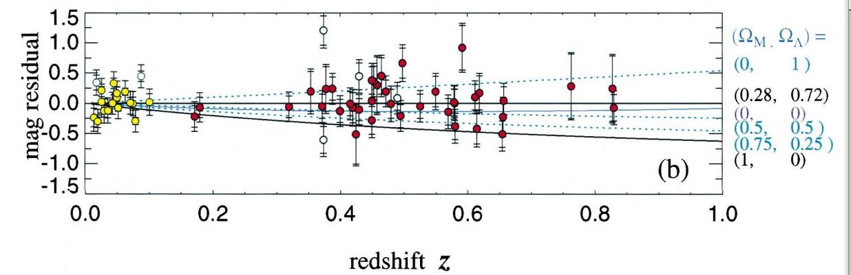
Figure taken from
Perlmutter et al., ApJ 517, 565 (1999)
So, what do we learn? What exactly is the value of ΩM?
In the years since the first announcements, astronomers have measured additional SNe Ia at high redshift, and continued to investigate systematic effects which can complicate this test.
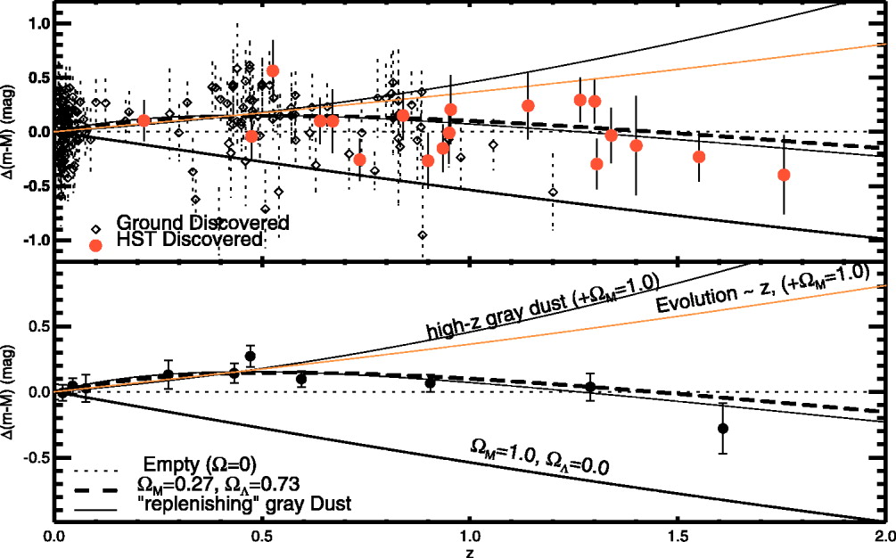
Figure taken from
Riess et al., ApJ 607, 665 (2004)
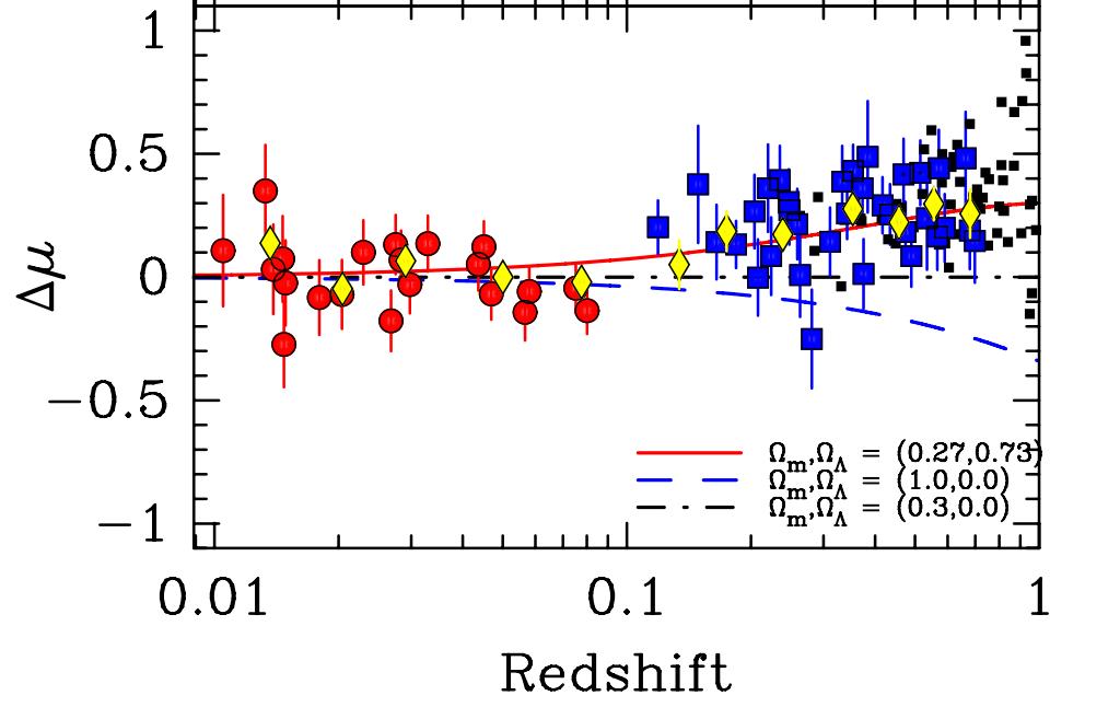
Figure taken from
Freedman et al., ApJ 704, 1036 (2009)
In order to understand these results, we will need to go back to the cosmological drawing board and see what happens if we dare to introduce a non-zero value for the cosmological constant Λ.
Copyright © Michael Richmond.
This work is licensed under a Creative Commons License.