 Copyright © Michael Richmond.
This work is licensed under a Creative Commons License.
Copyright © Michael Richmond.
This work is licensed under a Creative Commons License.
As astronomers gathered more and more examples of stellar spectra in the early twentieth century, they began to notice very subtle features. For example, one could classify stars into a relatively few spectral classes -- O, B, A, etc. -- on the basis of the relative strengths of common absorption lines. Within each class, one could find a small range of variation, and use it to define sub-classes: B0, B1, B2, down to B9. Fine.
But eventually, some of the classifiers noticed stars which fell into exactly the same class and sub-class -- say, A0 -- but which still showed some residual differences. Consider these three A0 stars:
In this part of the sequence, the spectral class is defined by several line ratios:
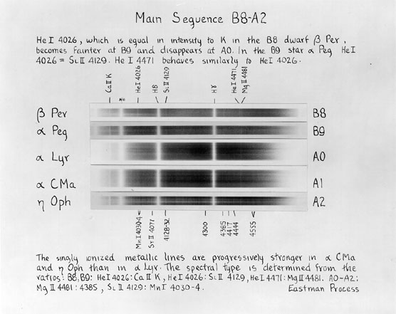
If we look closely at a small portion of the spectrum, we can verify that these line ratios are roughly the same in each:
But if we ignore the weak lines and look only at the very strong Balmer lines of hydrogen, we see an obvious change:
Exercise:
- What property of the Balmer lines changes?
- Estimate the magnitude of the change (5 percent? 10 percent?)
See also Figure 8.14 in your textbook.
In 1943, astronomers Morgan, Keenan and Kellman of Yerkes Observatory published a scheme for incorporating the width of absorption lines into stellar classification. Their book An Atlas Of Stellar Spectra defined the "MK" system. It used the same letters as the old Harvard system -- O, B, A, F, G, K, M -- and the same arabic numeral for subclasses based on line ratios -- A0, A1, A2, etc. -- but added another element: a roman numeral between "I" (one) and "V" (five). The higher the number, the wider the lines.
Note that this system was based on spectra recorded on photographic plates, taken with a camera attached to the Yerkes 40-inch refractor, as this excerpt from the Atlas describes:
A small one-prism spectrograph attached to the 40-inch refractor was used to obtain the plates. The reduction of collimator to camera is about 7; this makes it possible to use a fairly wide slit and still have good definition in the resulting spectra. The spectrograph was designed by Dr. Van Biesbroeck and constructed in the observatory shop by Mr. Ridell. The camera lens was constructed by J.W. Fecker, according to the design of Dr. G.W. Moffitt. The usable spectral region on ordinary blue-sensitive plates is from the neighborhood of K to H-beta (3920-4900 Angstroms).The dispersion used (125 A per mm at H-gamma) is near the lower limit for the determination of spectral types and luminosities of high accuracy. The stars of types F5-M can be classified with fair accuracy on slit spectra of lower dispersion, but there is probably a definite decrease in precision if the dispersion is reduced much below 150 A per mm.
Exercise:
- Calculate the entire length of the usable portion of a typical stellar spectrum on a photographic plate.
- Estimate the distance between the He I 4471 and Mg II 4481 lines on the plate
The full classification of a star in the MK system therefore looks something like this:
G2V A9III K4I
Note that sometimes one sees lower-case letters "a" or "b" appended to the luminosity class "I", like this:
K0Ia F2Ib
These are simply subdivisions of the luminosity class "I",
based on the widths of the lines.
What's going on? The basic idea is that the photospheres of some stars have much lower pressures and densities than others, even though the temperatures are the same. We'll deal with this idea in more detail later. It's enough for now to know that higher pressures lead to more collisions and broader lines.
So, the gas in some stars has much higher pressure and density than in others. Our Sun turns out to be one of the class "V" stars, with relatively high pressure and wide lines.
But what causes these variations in pressure?
The density of a star's atmosphere decreases as one moves farther out from the center. Near the center, it is extremely dense, complete opaque to any photon which might try to move through it. Very far from the center, the density decreases so far that photons can easily pass through it into space. Somewhere in between is a region where photons on average bump into just one more particle before escaping into space. We call this region the photosphere, the "visible surface" of a star.
Finding the exact location of the photosphere can be a little tricky -- it involves calculations of the optical depth that we will undertake next week. For now, let's assume that this critical point is defined roughly by the total number of atoms left "above" it. We could draw an imaginary cylinder reaching from the photosphere into space, like this:
Within this cylinder are all the atoms above the photosphere. We can simplify calculations by picking some height h at which the atmosphere becomes negligible, and then assuming that the gas is packed at some constant density ρ from the photosphere out to the top of the cylinder. The height h (very roughly the scale height of the atmosphere) is much, much smaller than the stellar radius, so this isn't a terrible approximation.
Can we find some relationship between the pressure of the gas at the base of this column (in the photosphere) and the "surface gravity" g at the location of the photosphere?
Exercise:
- The area of this imaginary cylinder is A. What is the mass of the gas within the cylinder?
- What is the gravitational force pressing down on the gas at the base of the cylinder?
- What is the pressure at the base of the cylinder?
Aha! The pressure of gas in the photosphere depends on the local surface gravity. The smaller g is, the lower the pressure, and hence the narrower the lines.
But why should stars have different values of surface gravity?
The surface gravity of a spherically symmetric star is simply
Exercise: Calculate the surface gravities of the Sun in cgs units, and compare it to the Earth's surface gravity.
Two stars with the same mass, but different sizes, will therefore have different surface gravities. Let's use the Sun as a fiducial star, and express the surface gravity, mass and radius in solar units. Then we have
Both mass and size play a role in determining surface gravity, but size is the more important player. Why? For two reasons:
Exercise: Calculate the surface gravities (in solar units) the following stars:
- Sirius A: mass = 2.0 solar, radius = 1.7 solar
- Sirius B: mass = 1.0 solar, radius = 0.008 solar
- Betegeuse: mass ~ 15 solar, radius ~ 600 solar
You've probably heard the terms "dwarfs" and "giants" applied to stars. Strangely enough, these adjectives don't simply describe the absolute size of a star; instead, they correlate more closely with the surface gravity, and, therefore, the luminosity class.
Actually, when you think about it, this isn't strange at all. The true size of a star is very difficult to determine; it involves finding the distance and the apparent angular size. The vast majority of stars in our galaxy are much too far away for us to measure these quantities even approximately. The luminosity class, on the other hand, can be determined from a single spectrum. Our current telescopes and detectors are sensitive enough to take the spectrum of any (unobscured) sun-like star in the Milky Way.
When one graphs the luminosity of a star against its temperature (in the "theoretician's version"), or the absolute magnitude of a star against its color (the "observer's version"), one finds that most stars fall within two regions of the figure:
The main sequence, running from lower right to upper left, consists of class V stars: dwarfs. The clump at upper right are stars with much lower surface gravities: red giants. The green lines show the locus of stars with a constant size. Note that most main-sequence stars are somewhere between 0.5 and 3 times the size of the Sun, while the red giants are 10 to 20 times larger.
The HR diagram above is based upon measurements of stellar distances made by the Hipparcos satellite. Since Hipparcos could only measure distances accurately out to about 100 parsecs, this diagram shows only a subset of the entire range of stellar types. Some stars are so rare that very few happen to exist within 100 parsecs of the Sun. If we extend our view to more distant reaches of the galaxy, at the expense of much larger uncertainties in luminosity, we must also extend the limits of our HR diagram.
Image courtesy of
www.anzwers.org
Note the scale at the top of the diagram: it shows the spectral class. The rough lines running through the diagram delineate the luminosity classes; they are simply drawn by hand based on the locations of individual stars of known type. Together, the spectral class and the luminosity class determine the (rough) location of a star in the HR diagram; and that, in turn, provides a (rougher) estimate of the star's absolute magnitude. In theory, we can use a star's spectral class as a guide to its distance:
This is called spectroscopic parallax, even though it doesn't involve any true parallax measurements. It ought to be called "spectroscopic distance", or something like that, but tradition can't be denied.
Exercise: According to SIMBAD, Deneb is spectral type A2Ia and has apparent magnitude V=1.25. How far away is Deneb?
Copyright © Michael Richmond.
This work is licensed under a Creative Commons License.