 Copyright © Michael Richmond.
This work is licensed under a Creative Commons License.
Copyright © Michael Richmond.
This work is licensed under a Creative Commons License.
The goal for today's exercise is for students who are interested in measuring an exoplanet's transit to practice their technique on a dataset I've acquired. These observations cover only a portion of a transit, and contain some ... questionable ... features, but the challenges may be a good preparation for the real adventure.
You will be analyzing a set of images which were taken at the RIT Observatory in March, 2026. The target is the WASP-149 system, which features a known Jupiter-size planet orbiting very close to its host star. The camera and observing parameters are the same as the ones students will use in this class for their own projects, so it should be good for practice.
You can grab a zip archive of the images from the link below.
Create a new folder/directory for this exercise, copy the archive into it, and unzip. You should find 80 raw FITS images: 20 darks, 20 flats, and 40 target images.
Midway through the analysis, you'll need to have a sub-folder to hold the cleaned version of these images. Please create a folder INSIDE your data folder, folder, with the name
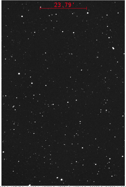
As a check that the files have been transferred properly, run AstroImageJ and open the file called wasp149_raw_0062.fit. It should look something like this:
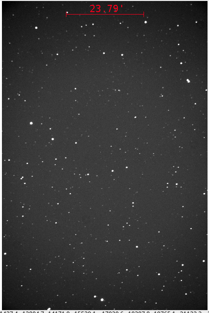
The image above has the standard orientation -- North up, East left -- which will match most charts. If your image looks upside-down, use the View -> Invert Y command to make it match this orientation. Be sure that all future work in this exercise adopts this same orientation.
There are twenty images with exposure times of 15 seconds, each taken with the lens cap covering the front of the telescope. These are "dark" frames, and the first step in the processing is to create a "master dark" frame using them.
Open one of the dark frames. In the image window, choose Process -> Data reduction facility .... The "CCD Data Processor" window will appear. We will give it a list of images to process, and tell it that it should "Build" a master dark image. Fill in the portions of the window shown below -- but replace the name of the folder in the "Filename Pattern Matching" box with the name of the folder on your computer which contains the raw images.
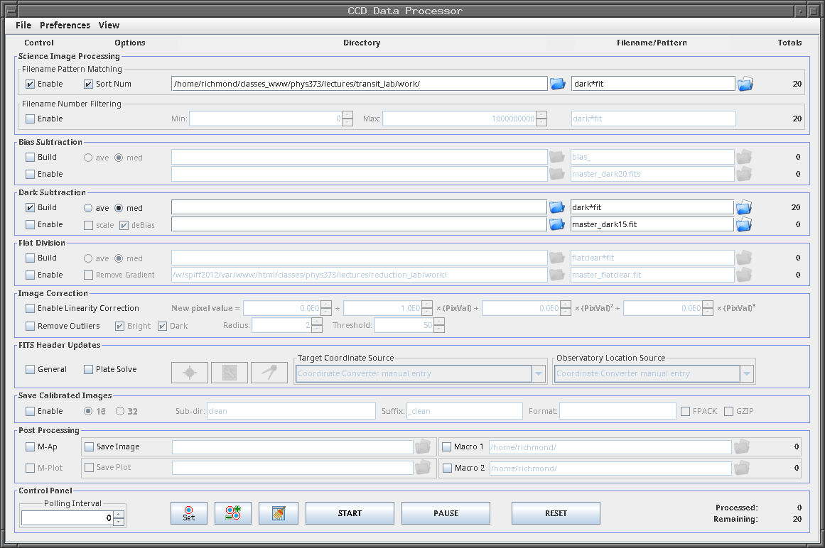
(Note that we choose the median option, rather than the average, when we create the master dark frame)
Click on the "START" button at the bottom to bring the procedure. After a short time, two new windows should pop up: a "Log" window should pop up, with a list of the operations it has carried out, and a new image window.
There should now be a new image in your folder, with the name master_dark15.fit. Open this image in a new window and verify that it looks reasonable.
We will use this master dark frame to process both the flatfield images and the target images, as our CMOS camera (ASI 6200MM) has a negligible dark current.
In addition to correcting for the "dark current", we'd also like to remove any variations in sensitivity across the focal plane. A perfect telescope and camera would respond to light equally in all locations ... but real telescopes tend to concentrate more light at the center of the image, and real cameras often suffer from the shadows of dust particles. In order to remove these effects, we create "flatfield images" by pointing the telescope at a blank white card, or a region of the sky at twilight. The result OUGHT to be a uniformly lit picture; we can use any deviations to gauge the sensitivity of each pixel, and remove it later.
I took a series of images of a white sheet of cardboard hanging on the inside of the dome. We'll use these to create the master flat.
AstroImageJ's "CCD Data Processor" window can do all this work for us. Open the window again, if necessary, and enter information as shown below. Again, replace the folder name in the Science Image Processing box with the appropriate folder on your computer. Note how we've modified the entry in the Dark Subtraction box from "Build" to "Enable"; that means that the master dark will be subtracted from each raw flatfield frame first, before they are all combined. Once again, we have chosen the median, rather than the average, when combining the images.
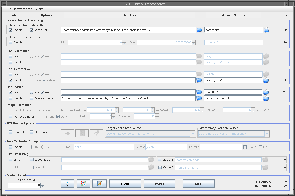
Click on the "START" button to create the master flatfield frame, which should have the name master_flatclear.fit.
We are ready to clean the target images. The procedure is
The "CCD Data Processor" window can do both steps at once and save the results in a new folder. Enter information in the window as shown below.
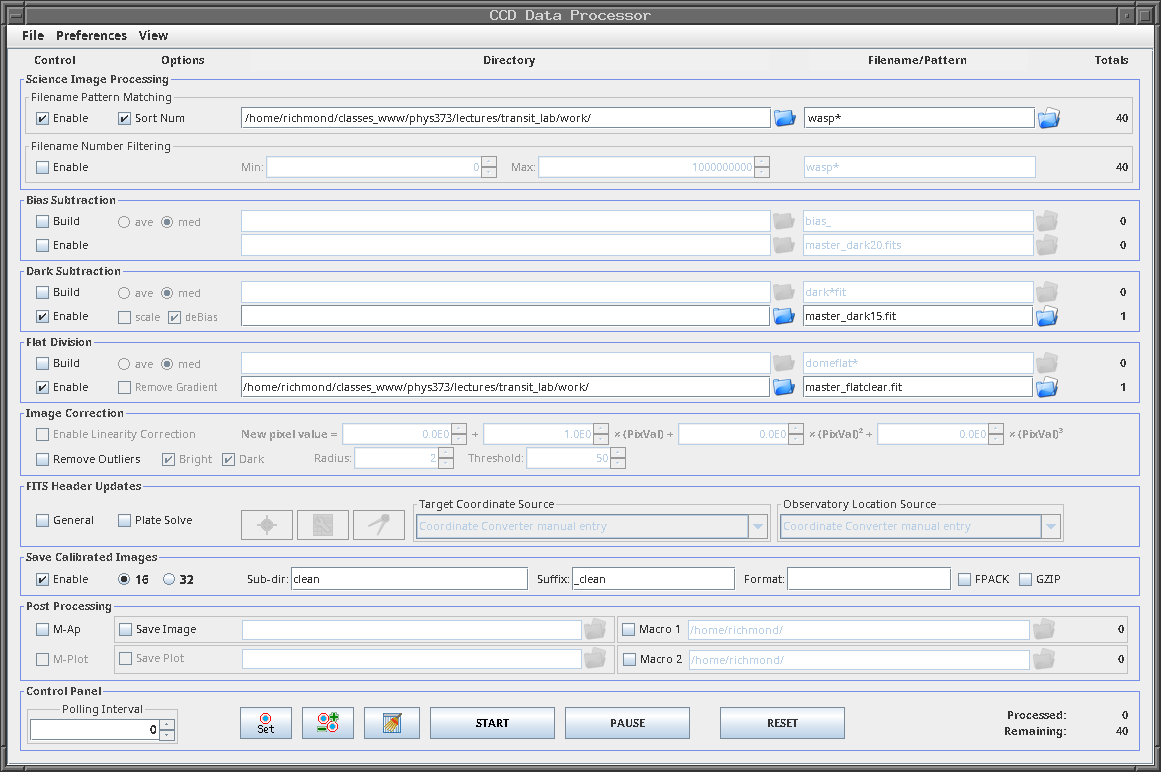
Click the "START" button and let AIJ do its work. When it has finished, open in the image called wasp149_clear-0062_clean.fits in the "clean" sub-directory. It should look nicer than the raw version:
Use the File -> Open image sequence in new window option to open all 40 of the cleaned target images in a single window. Use the slider bar under the image to scan through all of them quickly. Do you notice anything funny or strange about any of them?
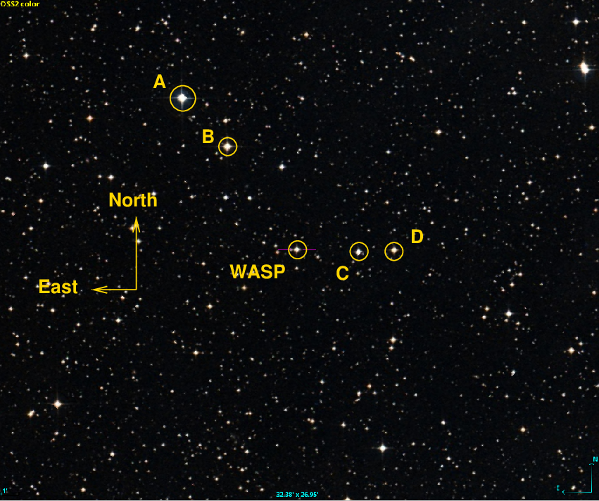
It's time to measure the brightness of the target star and four other stars on each of the images. The chart below identifies the target (WASP = T1) and the three comparison stars (A = C2, B = C3, C = C4, D = C5) that we will use.
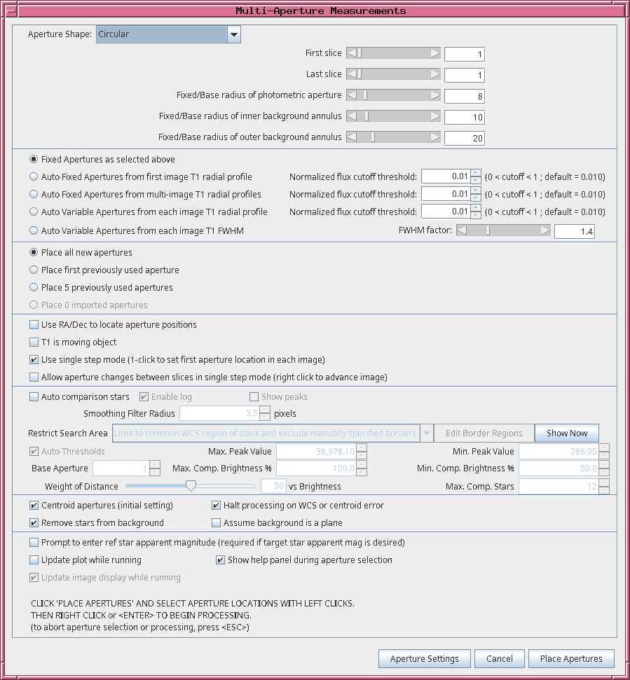
As we saw in the previous lecture, in order to perform aperture photometry properly, we need to choose the size of three circles:
I've determined that values of 8, 10, and 20 pixels, respectively, are appropriate for these images.
Run the image window's Analyze -> Multi-aperture command. A new window, "Multi-Aperture Measurements", will pop up. Fill in the blanks so it looks something like this:
It's time to measure the brightness of these five stars in all forty of the images. AIJ will do most of the work for us, we just have to give it a little guidance. Here's the basic idea: using the image window which shows one of the clean images,
In this way, we can quickly loop over a bunch of images, measuring the stars in each one. AIJ will save all the measurements in a single large spreadsheet file. Later, we can grab numbers from this spreadsheet to calculate relative magnitudes and make a light curve.
So, let's start. To simplify things, close all image windows. Now open a new image window to display the first clean image, in the clean folder.
Next, use File -> Open image sequence in new window to open all 40 of the clean images as a sequence in a new window. To do that, choose the first clean image, then, when the "Sequence Options" window pops up, enter "40" into the "Count" box (labelled "Number of images" in some version) and click "OK". The result should be a window with a set with forty clean images of the target. You can move the horizontal slider bar under the image to the left or right to display different images in the sequence.
Run Analyze -> Multi-aperture, and make sure that the "First slice" is set to 1, and the "Last slice" is set to 10. That will cause our measurements to run from the first to the last of the clean images.
Now click on the "Place Apertures" button at the bottom of the window. Indicate the locations of the target and the four comparison stars by
It's Show Time! You can begin the measurement process by clicking the right mouse button. A window called "Measurements" should appear, containing measurements from the first image.
In addition, a new image will appear in the window. All you need to do is indicate the position of the target star:
AIJ will figure out where all the stars are in this image, measure them, and write its results to the "Measurements" window. Afterward, it will again display the next image in the sequence.
Repeat this procedure in order to measure stars in all forty target images. All you have to do is left-click on the star "T1" in each image, and AIJ will do the rest.
When you have finished, the "Measurements" window should contain 40 rows. Use its File -> Save as command to save these measurements in a spreadsheet (.xls) file.
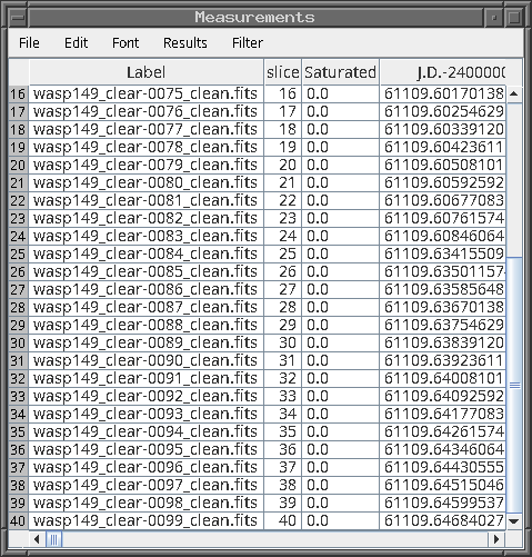
If you open the measurements file with a spreadsheet program, you should see many, many columns of numbers. The columns are separated from each other by "Tab" characters. The first few columns should look something like this:
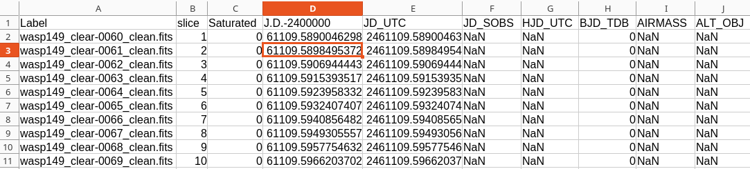
The columns of interest to us are the following.
  Value                column letter      column index
--------------------------------------------------------
   JD_UTC                 E                  5
   Source-Sky T1         AN                 40

   Source-Sky C2         BF                 58
   Source-Sky C3         BV                 74

   Source-Sky C4         CM                 90
   Source-Sky C5         DB                106
--------------------------------------------------------
It might be useful to copy these columns only into a separate file for convenience. If you can extract the data easily from the original file, that's fine, too.
Your last task is to create a light curve for the target star and the comparison stars. You can follow exactly the same methods you used back in
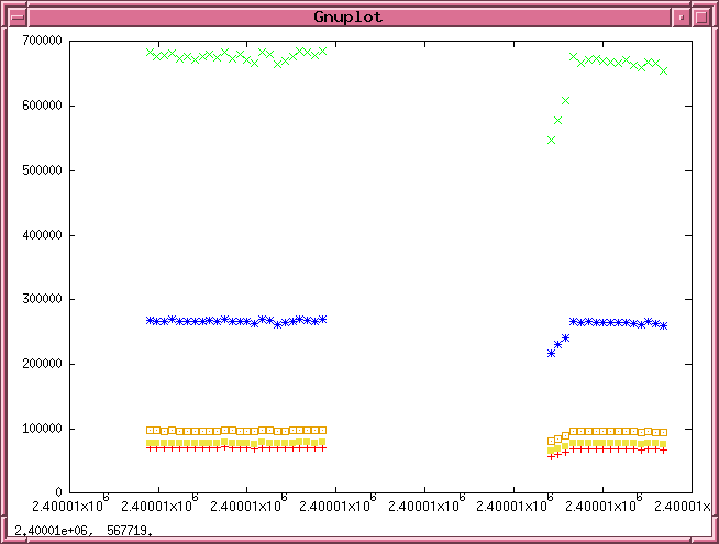
Begin by making a simple graph: the intensity of each star's light as a function of JD. It may help to subtract 2,461,000 (or some other large constant) from the JD values before plotting them.
What features do you see in this graph?
   Q:  Are there any gaps in the data?  If so, when do they start and end?
           What might have caused them?


   Q:  Do you see any trends which are common to ALL the stars?
           Can you provide any possible explanations for them?


   Q:  Should you discard any images?
One of the first things an astronomer should do is to examine all the measurements at once, in a big-picture view. It often reveals instances of good and bad measurements, outliers, and possibly bogus data which ought to be removed from further analysis.
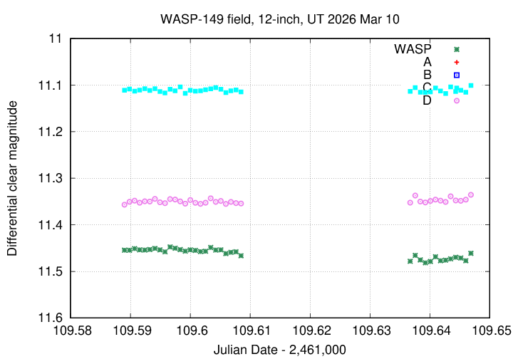
Now, exoplanet transits produce very small changes in the light of their host stars -- just a few percent at most. In order to see such small changes, you will need to perform differential photometry. Use any method you like to compute instrumental magnitudes from the intensity measurements, using the formula:
                                       [  Source-sky of star   ]
         instr_mag  =  9.0 - 2.5*log10 [ --------------------- ]
                                       [   Source-sky of C2    ]
Make a graph showing all five stars. The scale will probably be too large to show the very small variations expected for a transit.
So, make a second graph, modifying the vertical scale so that it runs from instrumental magnitude 12 (at the bottom) to 11 (at the top). This should zoom in on stars WASP, C, and D. Can you see any signs of a transit now?
Copyright © Michael Richmond.
This work is licensed under a Creative Commons License.