 Copyright © Michael Richmond.
This work is licensed under a Creative Commons License.
Copyright © Michael Richmond.
This work is licensed under a Creative Commons License.
Today, we look at the series of steps that one must carry out to measure the brightness of stars in a set of astronomical images. We can break these steps up into two groups:
Let's look at all the pieces in each group. You'll have a chance to put them all into practice on some real astronomical data in this week's lab exercise.
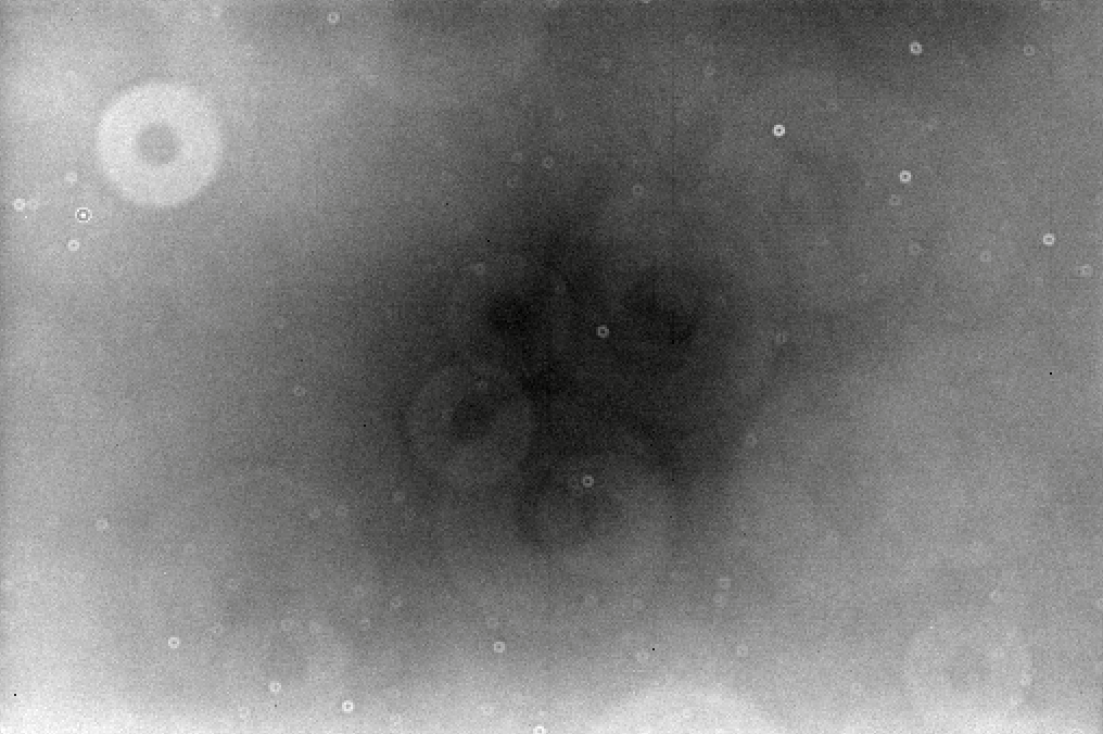
We'll work with a real set of images taken on the night of June 21, 2014. Here's one sample image of our target and a bunch of comparison stars. In its raw form, it's not pretty:
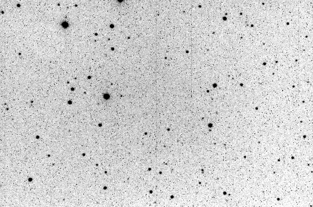
The big fuzzy blobs in this picture are the stars -- we want to measure them. But there are also a plethora of isolated hot pixels; yuck. You can see some vertical lines running through the middle of the image, too; those are due to defects in the silicon, causing the electron-transfer process between pixels to fail to some degree. Finally, you may note that the center of the image is considerably brighter than the corners.
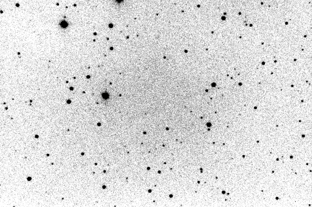
The procedure we'll describe below takes that awful, nasty, "dirty" image and turns it into a "clean" one like this:
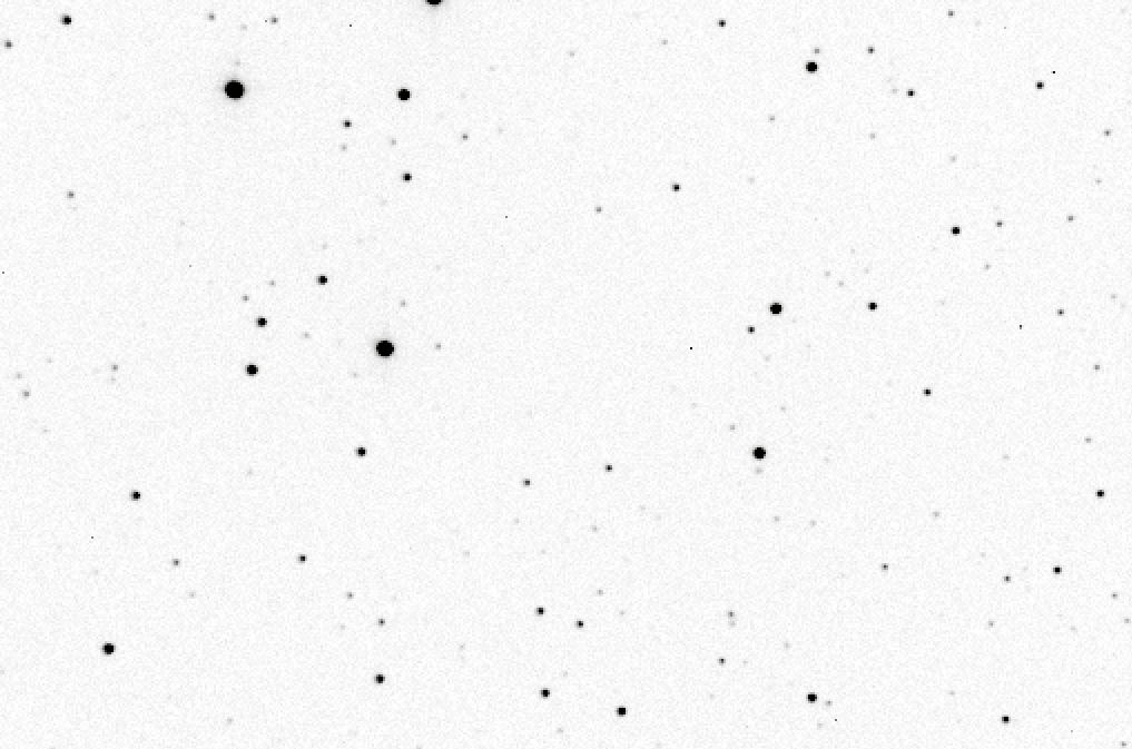
Isn't that nicer? Clearly, we can make better measurements of the number of photons which struck every pixel in this clean version of the picture.
The first step is to remove the "dark current" from each image. In theory, we could do this by taking a single dark image with the same exposure time as our target images. In this case, the target object's exposure time was 30 seconds. So, we might simply subtract one 30-second long dark image from each of the target images.
However, let's look at one 30-second dark image.
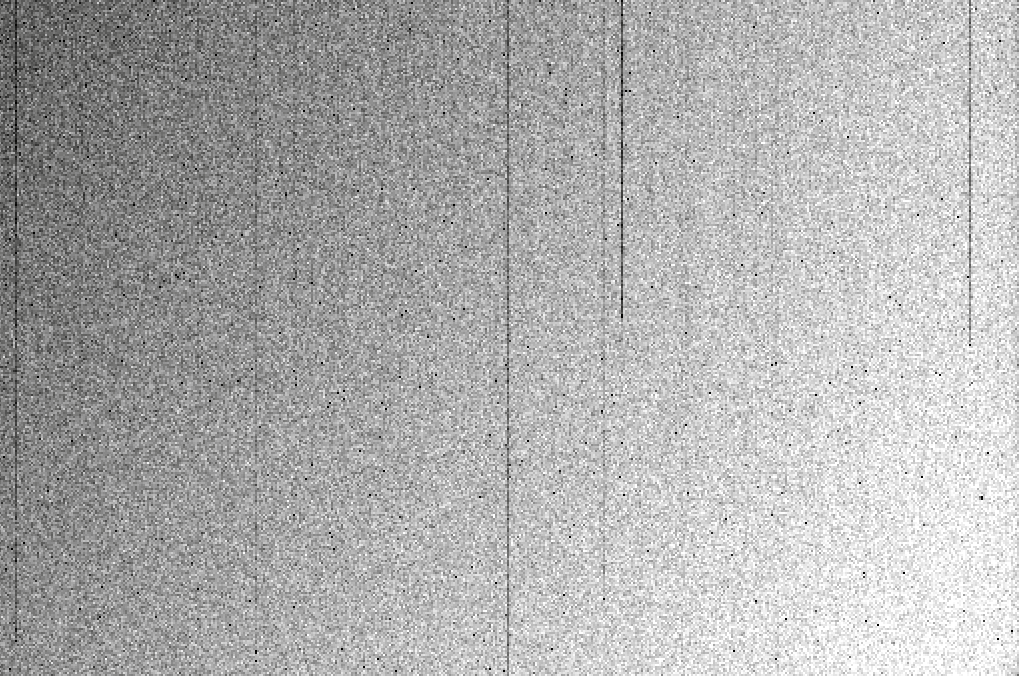
It shows those features we are hoping to remove, which is good. But it also shows something else: random variation. If we take a second dark frame, it looks similar -- but not identical. Each pixel has a slightly different value, just due to random fluctuations in the thermal jostling of neighboring silicon atoms. We could reduce that random variation by combining a bunch of individual dark frames.
A digression on "the best way to combine images."Suppose that you take a survey of incomes among a set of people who work in the Seattle area.
				Fred: $10,000
				Jane: $12,000
				Bob: $11,000
				Bill: $50,000,000
				Peter: $10,000
				Sally: $11,000
You want to describe the results of your survey with just a single number. What best represents the typical income of Seattle residents?
Perhaps you could use the mean, also called the average.
				Q: What is the mean of the 6 incomes?

				Q: Is that a fair way to describe the "typical" income?
A statistic which does a better job of ignoring isolated outliers is the median. It is simply "the number in the middle of the distribution." Here's how to calculate the median of a set by hand:
- sort the values
- count the values
- walk through the sorted array until you have gone past half the entries; then stop
- the current value is the median
If there are N elements in a set, then the median is just element number N/2 in the sorted set.
				Fred: $10,000
				Jane: $12,000
				Bob: $11,000
				Bill: $50,000,000
				Peter: $10,000
				Sally: $11,000


				Q:  What is the median of the incomes?

				Q: Does this seem more reasonable for the "typical" income?
Okay, back to images. If we take a set of dark frames, all with the same exposure time, then we create a "median dark image" in the following way. For each pixel in the image -- say, (25, 101) -- we collect the values of that pixel in all the images. Then, we compute the median. We place that median value into the pixel (25, 101) in our output image.
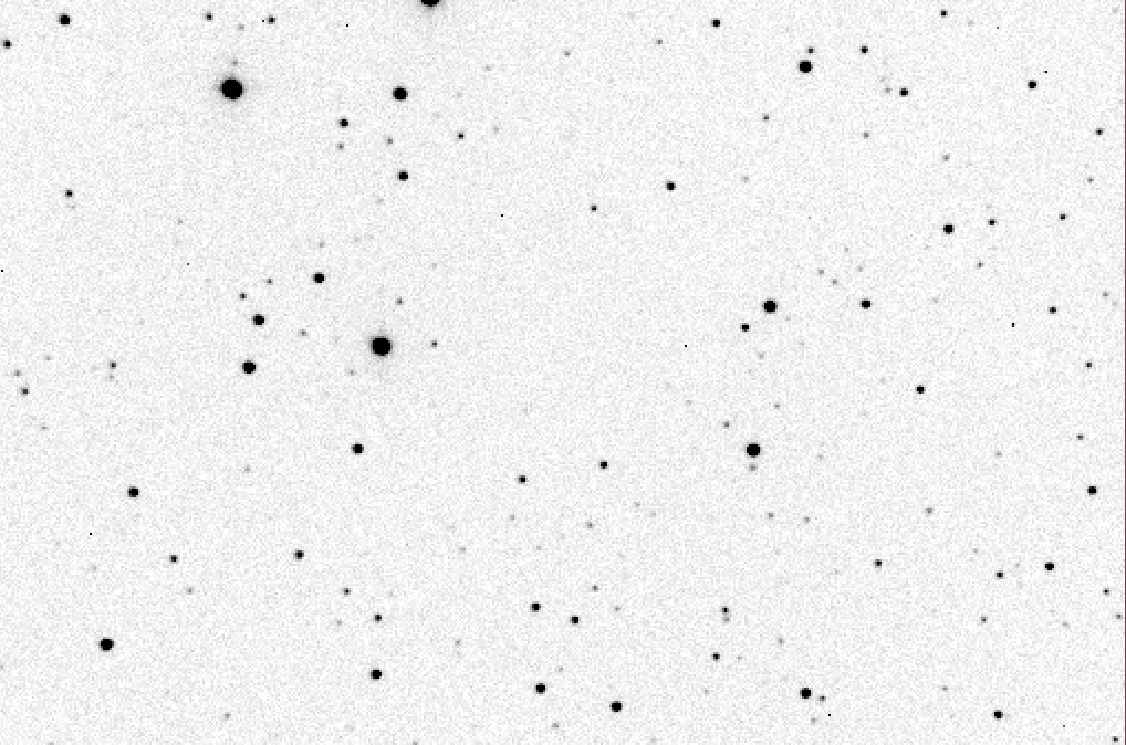
The result of taking the median of ten 30-second dark images looks like this:
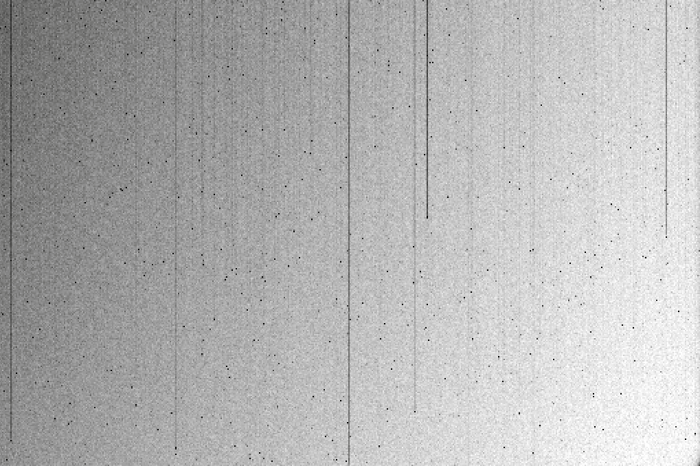
Notice how much smoother it looks. The bad columns are now much easier to pick out, and the hot pixels are easier to see, too.
It is necessary to create "master" dark frames for each different exposure time in your dataset. So, for example, you might have a master dark for images with exposure time of 1 second, and another master dark for images with an exposure time of 30 seconds.
In order to correct for variations in sensitivity to light across the focal plane, astronomers take a picture of some uniform source of light; it could be the daytime sky, or it could be a white card on the interior of the dome. This picture SHOULD show a uniform, blank field of light, but in practice, rarely does. Instead, it shows a pattern like this:
![]()
Exactly these variations ought to be present in all target images taken with the same optical system. We can correct for them by dividing the images by this flatfield.
However, we can't just take a single flatfield image and divide our target images by it. We need to create a proper "master" flatfield image in the following way:
The resulting "master" flatfield image will have a lower random noise contribution than any single flatfield image. Compare the median of ten flatfield frames, shown below, to the single flatfield frame above.
One last thing before we're finished with the master flatfield frames. Our plan is to divide the target images by the appropriate flatfield. Well, if the typical pixel value in the flatfield is 8000 (a picture of a brightly-lit white card) and the typical pixel value in a raw target image is around 1000 (a picture of the dark night sky), then the result will be something like
         raw target pixel        1000
        ------------------  =  --------  =   0.12
         master flat pixel       8000
Whoops. All the pixels in our target image will have teeny tiny values, much less than one. That's not good.
To avoid this problem, we can normalize the master flatfield frame. It's simple to do: compute the mean value of the master flatfield frame, and then divide the master flatfield frame by that mean value. If three neighboring pixels in the master flatfield frame had values of
8010 7965 8025
then after dividing each by the mean value of 8000,
we'll end up with pixel values of
1.0012 0.9956 1.0031
In other words, all the pixels in the master flatfield will become very close to 1.0. When we divide the target frame by this normalized flatfield, the result will be a target frame with the same typical pixel value as it originally had -- but without the variations in sensitivity.
Right. Once we have all the master darks and master flats, we can clean our raw target images. The method is pretty simple. Start with one raw image.
First, we subtract the appropriate master dark frame from each raw image.
Second, we divide by the normalized master flatfield frame.
Ta-da! We have finished the cleaning portion of the reduction.
Astronomers call the measurement of light photometry. Over the years (and decades, and centuries), we have developed many different techniques, each suited for particular situations. The method we will use in this class is called sythetic aperture photometry,
We can illustrate this method with an image of the galaxy M74.
![]()
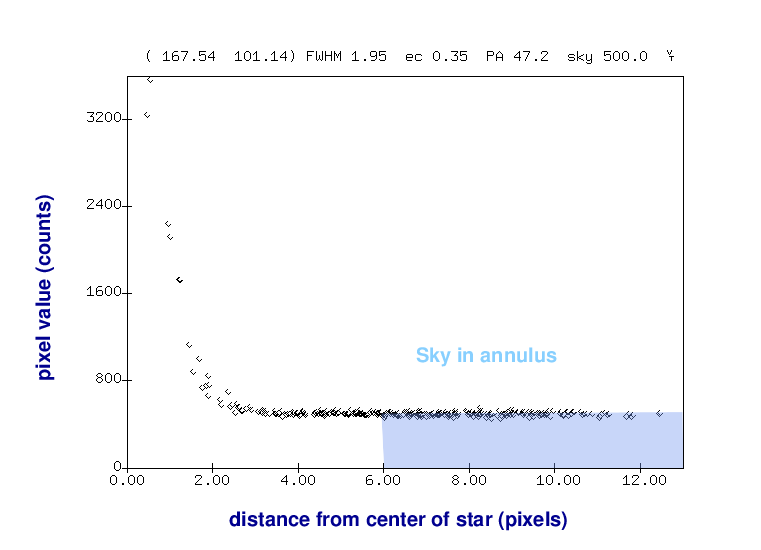
Suppose we want to measure the brightness of one star, the bright one to the lower-right of the galaxy's bulge. We can get a feel for the quantitative pixel values near this star by making a radial profile plot of the star. On the horizontal axis is the distance of each pixel away from the center of the star, and on the vertical axis is the pixel value above the local sky value.
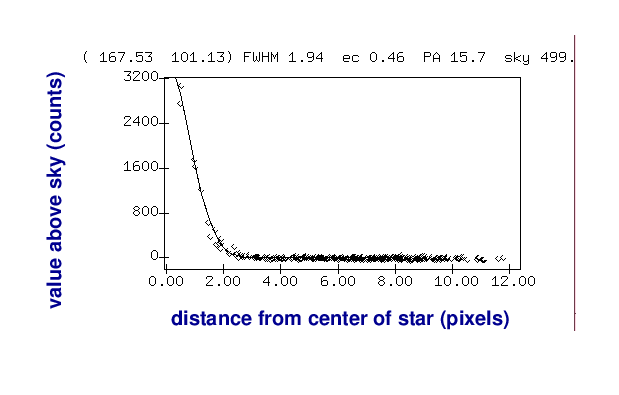
One very simple method is just to pick the largest pixel value in this graph:
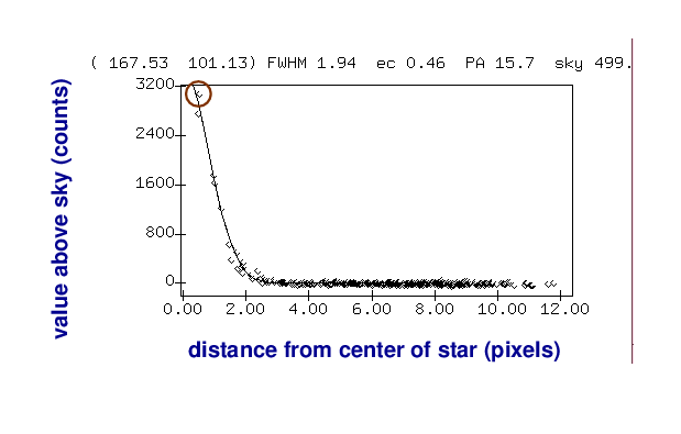
As you can imagine, this isn't very accurate for several reasons. Depending on the exact position of the star on the CCD, the peak of the point-spread-function (PSF) might fall at the center of the pixel, or near the edge, or even near the corner; the amount of light recorded by that pixel would vary in each case.
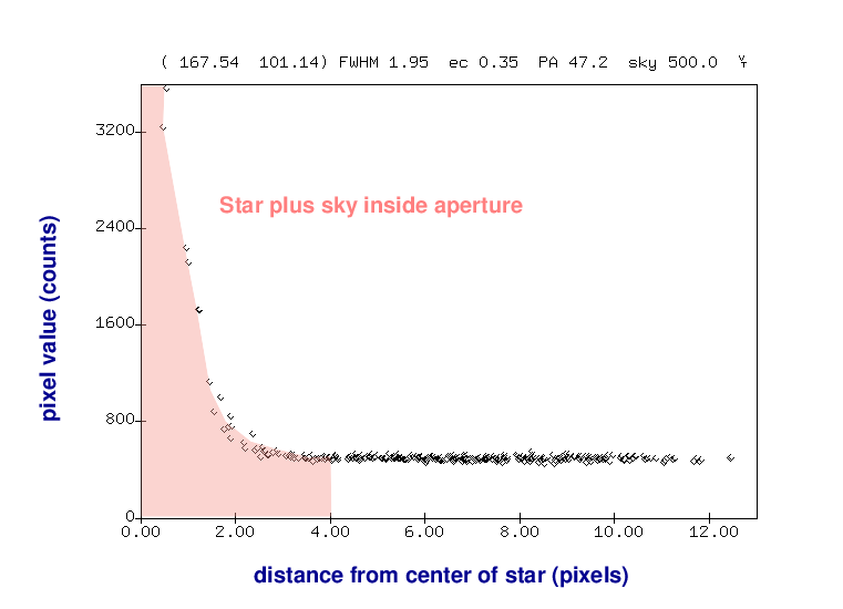
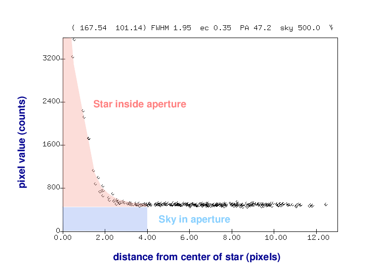
A better approach is to add up all the light which falls onto the CCD within a small region around the center of the star:
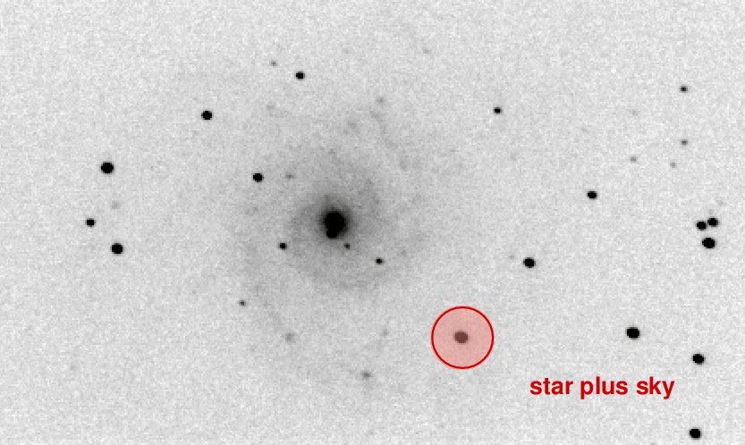
Of course, that will mean that we include some light from the sky as well.
But we can then use an annulus around the star to measure the typical sky value, without any contamination from the star's light.
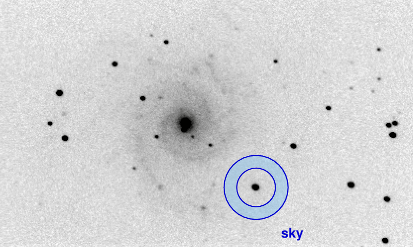
Once we know the local sky value, we can go back to our measurement of light inside the aperture and remove the contribution from the sky -- leaving a good measurement of the light from the star, all by itself.
Note that in many astronomical images, the general background value changes from one location to another. In our example picture of the galaxy M74, a star at location "A" would be mixed with much more background light than one at "B" or "C".
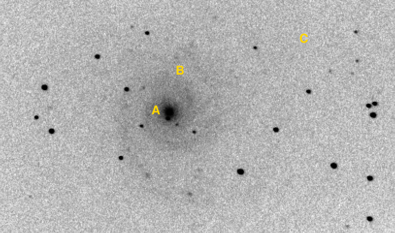
Defining a "local" sky value at the location of each star allows us to subtract that background contribution most accurately.
In order to make the best measurement, we need to choose the right sizes for these three circles:
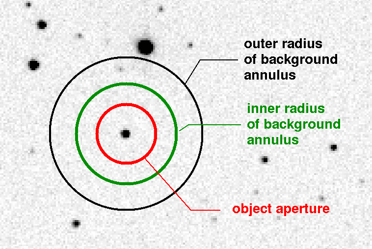
Some reasonable rules are
After all the work we've done so far, this last part isn't so difficult. For each star in the image, we determine its exact central location, and then follow these steps.
This method of measuring light from a star will give much better results than simply finding the brightest single pixel. With proper choices for the sizes of the apertures, and a careful accounting for the pixels which lie partly inside and partly outside each circle, synthetic aperture photometry can yield measurements accurate to fractions of one percent.
Of course, as you have seen in past exercises, it's not enough to measure the light of a single star to make a good light curve. Usually, you must measure the light from several other comparison stars as well, in order to detect and correct for image-to-image changes in transparency, seeing, or other systematic factors. A good software package will allow you to define a number of apertures, designate the positions of a set of stars, and then carry out the measurements on all those stars, in all the images.
Copyright © Michael Richmond.
This work is licensed under a Creative Commons License.