 Copyright © Michael Richmond.
This work is licensed under a Creative Commons License.
Copyright © Michael Richmond.
This work is licensed under a Creative Commons License.
Today, we use the CMB in order to measure the rate at which the universe is currently expanding; in other words, we see how the CMB can be used to find H0. The good news is that, with a bit of work, it can be done. The bad news is that the value we find is (currently) NOT the same as the value determined by our regular old distance-ladder method.
Most of this course has focused on methods for measuring distances to objects in space. It's a difficult job, in general, and so we adopted a method called the "distance ladder:"
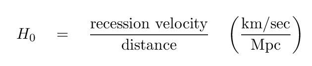
Once we know the distances (and velocities) of some very far-away objects, we can calculate the Hubble constant:
Astronomers who study the cosmic microwave background, on the other hand, are looking at radiation which has travelled a long, long, long way through space to reach us: the CMB is the MOST DISTANT object we can observe. Some scientists have figured out a very different approach to finding the value of the Hubble constant: rather than starting close to the Sun, and working outward to more distant regions, this methods starts with the CMB and works INWARD towards the Sun. For this reason, it is sometimes referred to as "the inverse distance ladder".
Let me try to explain the basic idea behind this completely different method for measuring distances. I'm no expert at it, so I may make some mistakes.
Way back in the very early universe, when it was still so hot that all the matter was ionized, there was a mix of dark matter, baryonic matter, and photons (and neutrinos, but we'll ignore them for now). Overall, the density of this mixture was relatively uniform; but there were some places which were a little more dense than usual, and some which were a bit less dense.
The overdense regions generated regions of higher pressure. The dark matter simply settled into the center of each dense region, because it interacted with the rest of the mixture only via gravity; but because the baryonic matter (gas) and photons could push and pull each other via electric forces, they reacted to pressure by expanding outward. So, around each overdensity, a wave of (gas + photons) spread out at the speed of sound. Because the gas was ionized, it was opaque, and trapped the photons; the gas "went along for a ride" as the photons spread outward.
Animation courtesy of
Ned Wright's Cosmology Pages
When the temperature of the universe dropped to about 3000 degrees or so, the electrons and protons combined to form neutral hydrogen -- which is transparent to most radiation. Suddenly, the photons could pass through the gas and fly off on their own.

The baryonic matter was left sitting in a big shell around the dark-matter core of each overdense region.
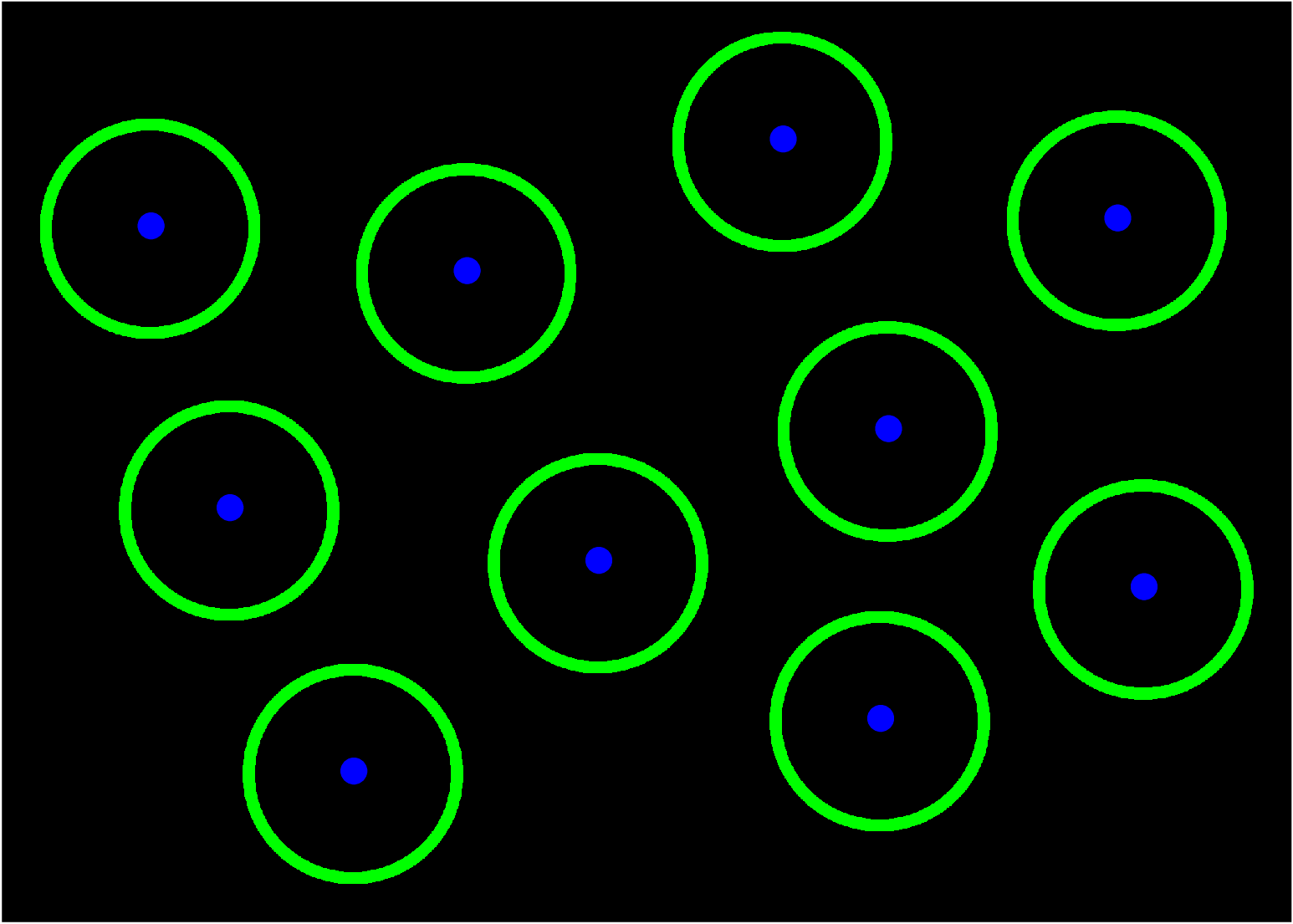
The result: a very young universe in which there are a bunch of "nuggets" of dark matter, each surrounded by a shell of baryonic matter of a roughly similar size.
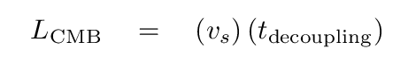
Q: Estimate roughly the radius of these shells of higher density.
The shells should have a size
The escaping photons carry with them a ghostly picture of these shells -- and that's what we see when we examine the Cosmic Microwave Background closely.
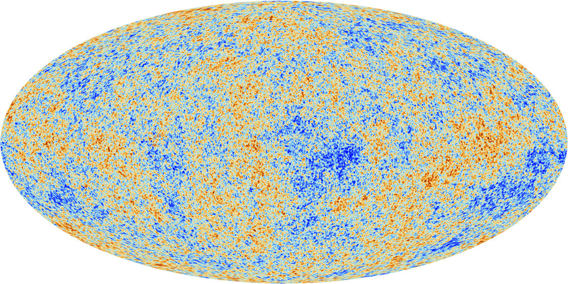
Image courtesy of
ESA and the Planck Collaboration
If we could watch the universe evolve in time, those shells of higher density would form more galaxies than the less-dense regions around them. As a result, we expect to see many galaxies separated by distances equal to the radius of the shells.
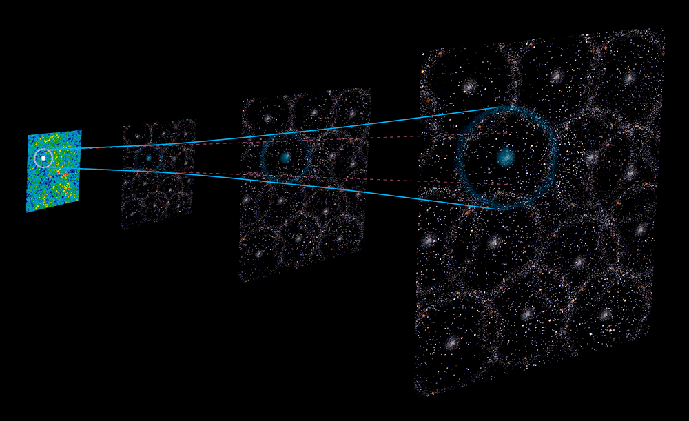
Image courtesy of
Gabriela Secara, Perimeter Institute
One way to measure the size of these shells in the early universe is to compute the power spectrum of the fluctuations in the CMB. The big bump is the "first acoustic peak", which corresponds to angular size of the shells.
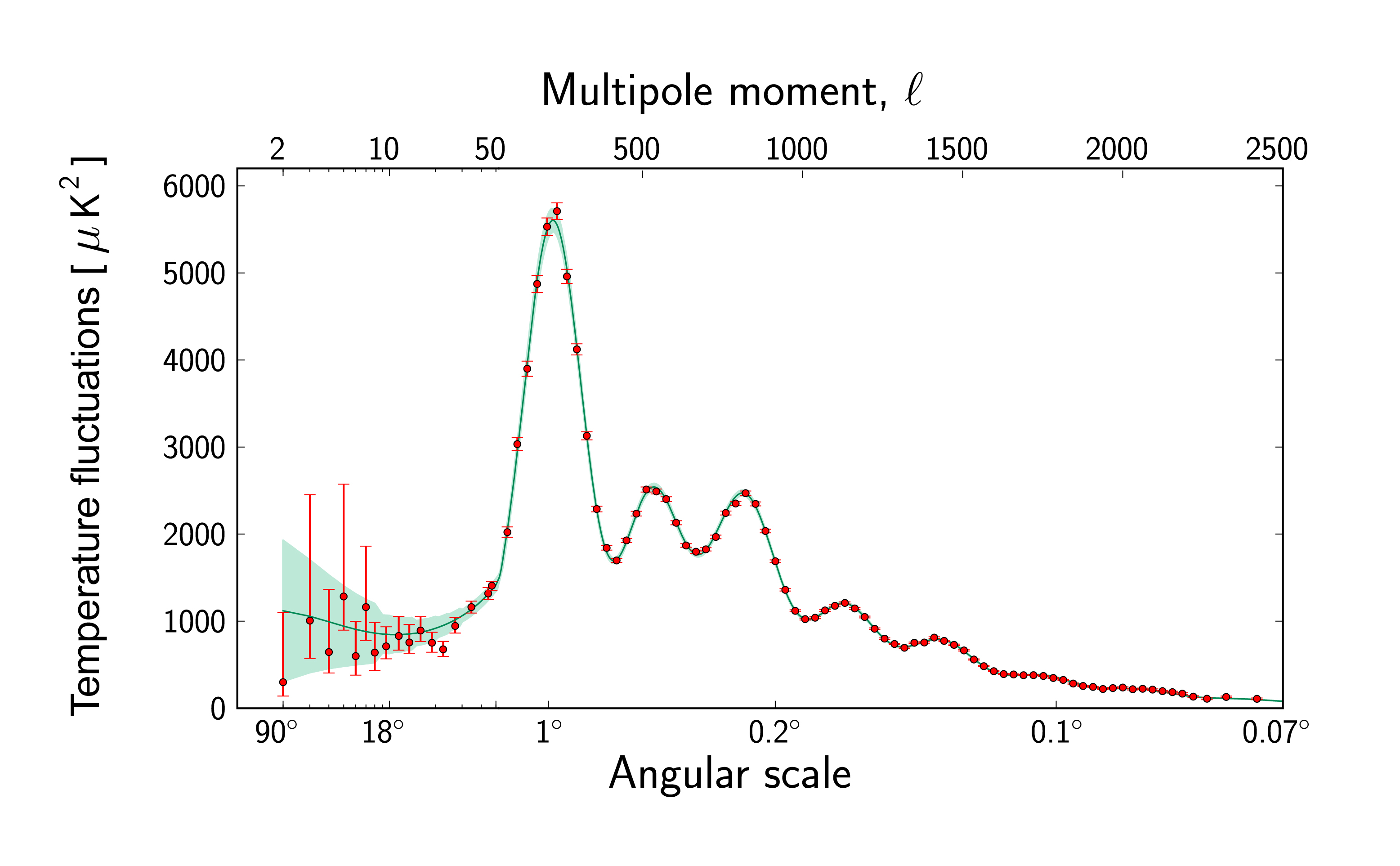
Image courtesy of
ESA and the Planck Collaboration
The remnants of these shells provide a "ruler", which can be identified in the modern-day universe by measuring the separation between pairs of galaxies. If our theories are correct, there should be a special angular distance between galaxy pairs which is very common. We can look for that special angle by computing the two-point correlation function of galaxies.
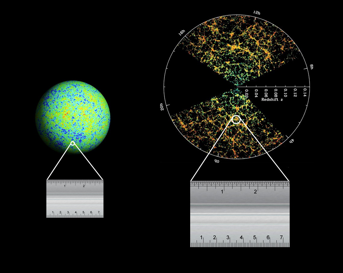
Image courtesy of
NASA’s Wilkinson Microwave Anisotropy Probe, Sloan Digital Sky Survey,
and Laurence Berkeley Laboratory
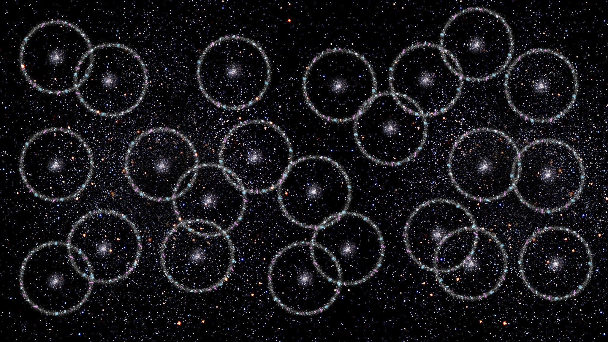
Image courtesy of
Gabriela Secara, Perimeter Institute
Evidence for these ghost-shells in the local galaxy population was first detected by the SDSS survey back in 2005.

Figure 2 of
Eisenstein et al., ApJ 633, 560 (2005)
and confirmed by later surveys.

Figure 16 of
Anderson et al., MNRAS 427, 3435 (2012)
So, how does this help us to measure distances? Again, I'm not an expert in this technique, but I believe that it goes something like this:

Now, in practice, we need to include galaxies within a range of redshifts (say, 0.45 to 0.65) in order to create a sample large enough to show the bump in the 2-point correlation function due to the shells; that introduces some uncertainty in our calculations. The measurements of the angular sizes have some uncertainty as well, as do the other calculations mentioned in this procedure above. A recent paper shows the diagram below to indicate how one can fit models of the universe's expansion to the BAO data (shown as blue symbols) to determine the value of H0 at the current time. As you can see, the BAO measurements have pretty large uncertainties, due in part to the relatively small volume of space and small number of "shells" within that space.

Taken from Figure 1 of
Cao et al., Universe, 7, 57 (2021)
Q: What is the value of the Hubble constant right NOW, at redshift z = 0?
Yes, the best estimates of H0 using this CMB-based technique are clustered quite tightly around H0 = 67 km/s/Mpc.

Modified slightly from Figure 2 of
Cao et al., Universe, 7, 57 (2021)
The ordinary distance ladder allows us to build outward, using several different methods to extend our reach. The most common method of measuring H0 involves observations of Type Ia supernovae, since they are luminous enough to be detected at very large distances. Of course, this is a complicated process which involves a number of different steps.
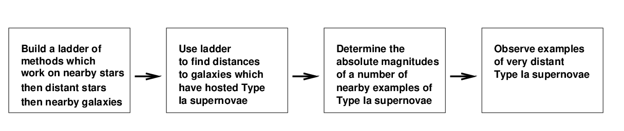
One of the groups which has worked on this method in recent years is the Sh0es collaboration, led by Adam Riess. This project has chosen Cepheids as the key rung in their distance ladder: they have measured many, many Cepheids in a number of nearby galaxies which hosted type Ia supernovae. Using the Cepheid-based distances to these host galaxies, the team has computed the absolute magnitudes of (a sub-group of) Type Ia supernovae, and then compared that to the apparent magnitude of very distant (and faint!) Type Ia supernovae in order to calculate distances.
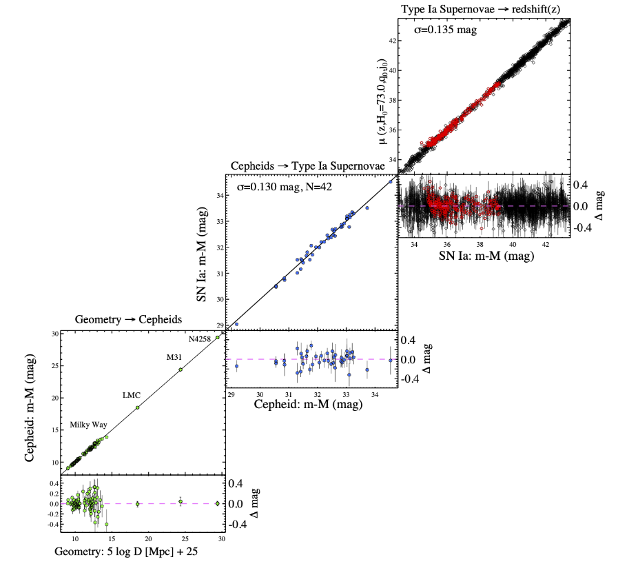
Figure 12 taken from
Riess et al., ApJ 934, 7 (2022)
The value of H0 determined by the Sh0es team is roughly 73 km/s/Mpc.
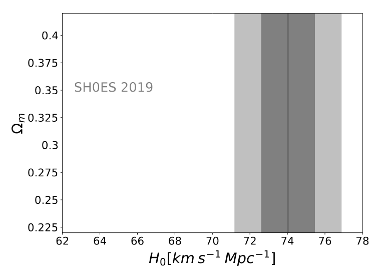
Modified slightly from Figure 2 of
Cao et al., Universe, 7, 57 (2021)
Q: Is this the same as the value determined via the inverse distance ladder?
Alas, no. The ordinary distance ladder and the inverse distance ladder yield different values. What's worse is that they don't even agree within the uncertainties!
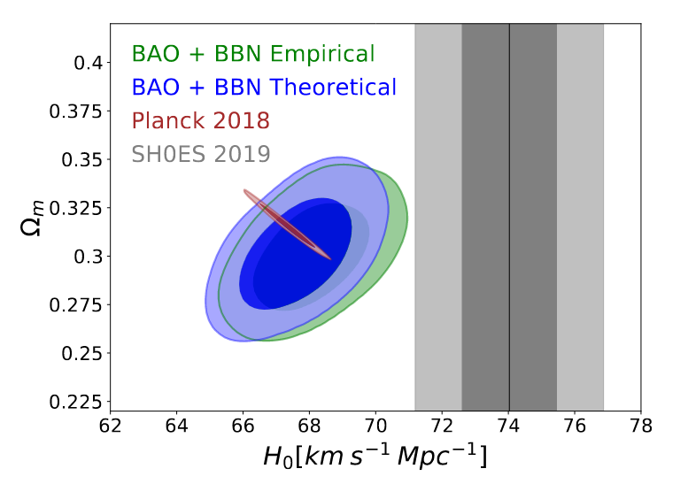
Figure 2 of
Cao et al., Universe, 7, 57 (2021)
Now, there are a (at least) couple of possible explanations, some or all of which could be true.
If the entire universe is homogeneous, the properties of LOCAL and OBSERVABLE should be the same. But if there are small differences between one portion of the observable universe and another -- if, for example, one region is slightly more dense, and another is less dense -- then the expansion rates within those regions will be slightly different.
But what if that's not right? What if, for example, the cosmological constant ... isn't constant? Observations made by the Dark Energy Survey Instrument (DESI) collaboration over the past decade, and released in the past year, suggest that Λ may change over time. The extracts from one of their papers below use slightly different language to describe this property of space: in their terms, w0 = -1 and wa = 0 means that Λ is constant ... but other values mean that Λ changes over time.
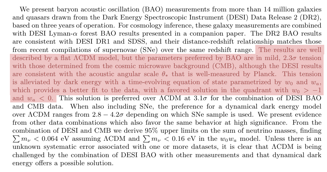
Abstract taken from
DESI DR2 Results II: Measurements of Baryon Acoustic Oscillations and Cosmological Constraints ,
arXiv 2503.14738 (2025)
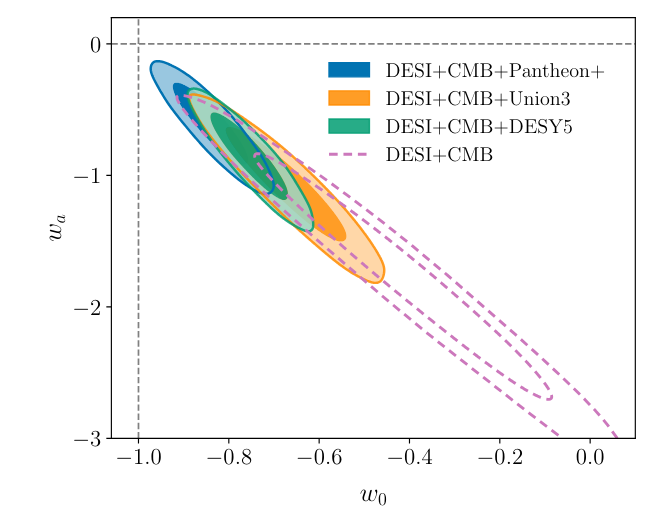
Figure 11 taken from
DESI DR2 Results II: Measurements of Baryon Acoustic Oscillations and Cosmological Constraints ,
arXiv 2503.14738 (2025)
Copyright © Michael Richmond.
This work is licensed under a Creative Commons License.