 Copyright © Michael Richmond.
This work is licensed under a Creative Commons License.
Copyright © Michael Richmond.
This work is licensed under a Creative Commons License.
Our goal in this class is to study objects which lie outside our own Milky Way Galaxy. However, the methods we've covered so far won't do the trick. Parallax, for example, even with the latest Gaia release, can't even reach to the center of our galaxy -- let alone beyond it.

Last time, we investigated how we might try to use the parallax measurement to one star in order to estimate the distance to a "twin" which might lie much farther away. The method yields inconsistent results, due in large part to the difficulty of identifying an exact match to the nearby star.
Today, we take that approach and improve it by using not just one, but hundreds or thousands of stars simultaneously to serve as the "nearby" and "distant" objects. The key is to choose stars which are members of a single stellar cluster.
Using just one nearby star to determine the distance to one distant star is not easy, as we have seen. A better idea is to pick a BUNCH of local stars, and a BUNCH of distant stars, and compare the properties of these two groups to determine the relative distance between them. If we pick the groups carefully, we can address some of the problems that we encountered when trying to match single stars. Remember these?
All we need to do is to make one assumption:
     Assume: All the stars in a cluster are born at the same time
             from a cloud of gas which has uniform chemical composition.
With this proviso, the members of an open cluster or globular cluster provide us with an excellent set of subjects, one which reveals quite a bit about its age and metallicity.
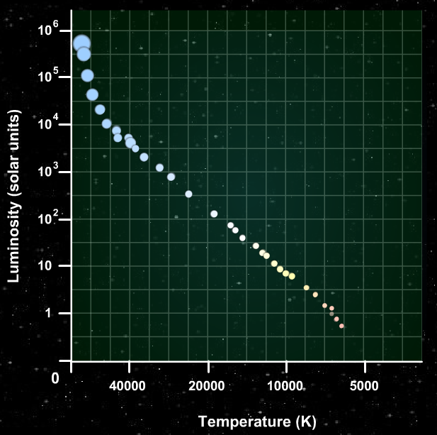
When the stars are first born, they all lie on the main sequence of a Hertsprung-Russell (HR) diagram. Massive stars are hot and luminous, low-mass stars are cool and feeble. (Click on the figure below to activate it)
After 5 million years, the most massive stars run out of hydrogen in their cores and leave the main sequence, moving toward the red giant area of the HR diagram.
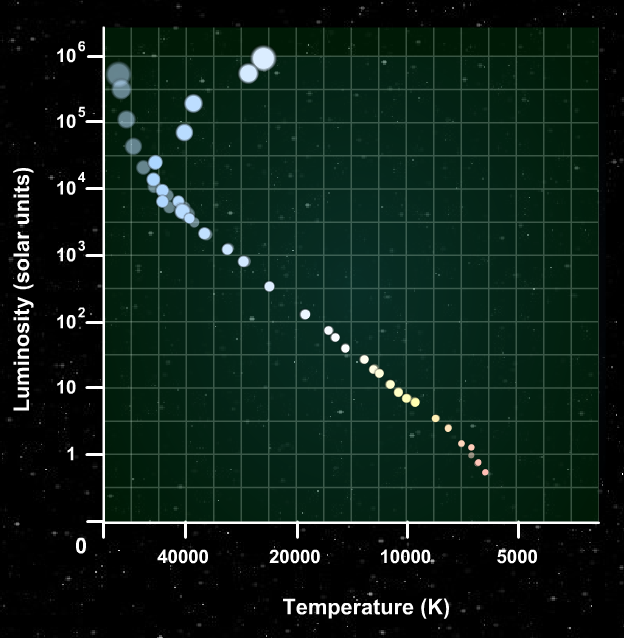
After 80 million years, the most massive stars are long since dead. Now less massive stars start to evolve off the main sequence ...

And after billions of years, only the low-mass members of the cluster remain on the main sequence.

So we can estimate the age of a cluster of stars by looking at the location of the main-sequence turnoff on its HR diagram.

Image taken from Fig 3 of
Feuillet, Paust and Chaboyer, PASP 126, 733 (2014)
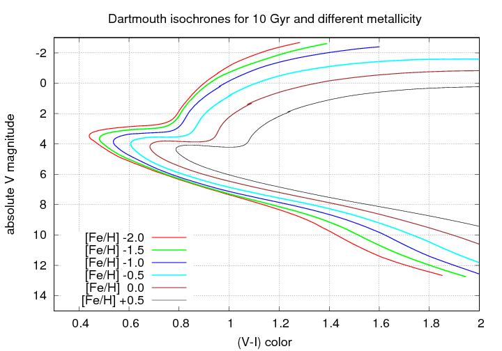
The change in shape of the HR diagram with age is pretty straightforward, but also relatively small after a few billion years. For globular clusters, for example, which typically have ages greater than 8 Gyr, look at the change with time; the figure below is based on isochrones (models of stars created with a particular age and metallicity) provided by the the Dartmouth stellar evolution group.
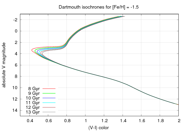
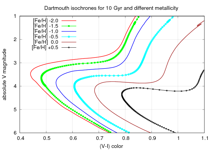
Let's zoom in to see more closely the region of the main sequence turnoff point:

But age isn't the only variable which can affect the luminosity of the stars in a cluster: the metallicity of the gas making up the stars can also have an important effect. A good illustration of this point is given by Ross et al., AJ 147, 4 (2014). In their Figure 8, they show color-magnitude diagrams for 5 globular clusters with a range of metallicities, ranging from the very metal-poor M92, [Fe/H] = -2.3, on the left, to the metal-rich NGC 6791, [Fe/H] = +0.4, on the right.

Figure 8 taken from
Ross et al., AJ 147, 4 (2014).
  Q:  What features in these HR diagrams
      change with metallicity?
I can see at least three pretty obvious features:
Note that the first feature, the color of the turnoff point, can be affected by reddening; so one has to be very careful to measure the extinction to the cluster properly. But the other two indicators are relatively reddening-independent, which makes them easier to apply in many cases.
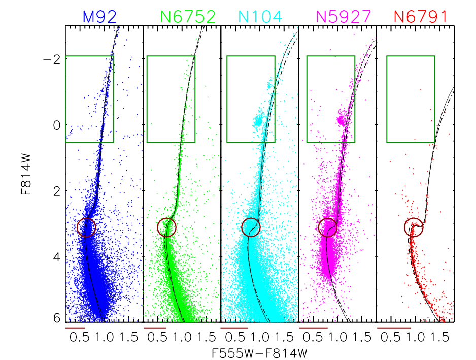
Figure 8 taken from
Ross et al., AJ 147, 4 (2014).
The graphs above don't show the horizontal-branch components very clearly. One can see the effects of chemical composition on the horizontal branch more clearly in data presented in Gaia Data Release 2: Observational Hertzsprung-Russell diagrams .
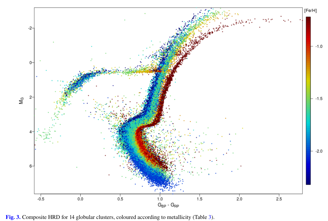
Image taken from Fig 3 of
Gaia Collaboration et al., A&A 616, A10 (2018)
The authors of the paper compare the main-sequence turnoff point to a number of isochrones with different metallicity. What short of changes occur in the HR diagram of a cluster as a result of metallicity? Let's take a look:
That's a much larger change than we saw with ages. Again, let's zoom in to look at the main-sequence turnoff point:
In the figure below, which uses a color based on the HST F390M and F555W filters, which is similar to (B-V), you can see the location (in color) and shape of the main-sequence turnoff change very clearly with metallicity. The solid black lines in the diagram are isochrones from the Dartmouth stellar isochrones; the model for M92, for example, has an age of 13.5 Gyr and a metallicity of [Fe/H] = -2.3.
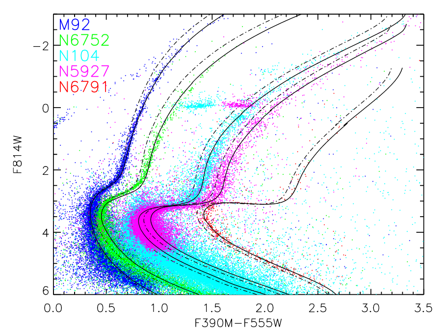
Figure 11 taken from
Ross et al., AJ 147, 4 (2014).
So, if we measure the properties of a large number of stars in a single cluster, then we can use the HR diagram to figure out the age and metallicity of all the stars in the cluster.
Then, if we find another cluster with similar properties, we can safely use the offset between some feature in the HR diagram to measure the relative distance between the clusters.
If you study clusters in detail, you'll want some way to convert the observed properties (magnitudes and colors) into physical properties of the stars (ages, masses, metallicities). Computing stellar models is a complicated business, so it makes sense to use the results of experts.
The Darthmouth Stellar Evolution Database provides you with a web-based interface that allows you to generate models according to your own preferences, then download the resulting isochrones. Let's give it a try to see how this works.
First, go to the The Darthmouth Stellar Evolution Webtools webpage. You should see a page like the one below.

You should receive shortly a small ASCII text file. Download it to your computer, and examine it with any text editor. You'll see something like this:
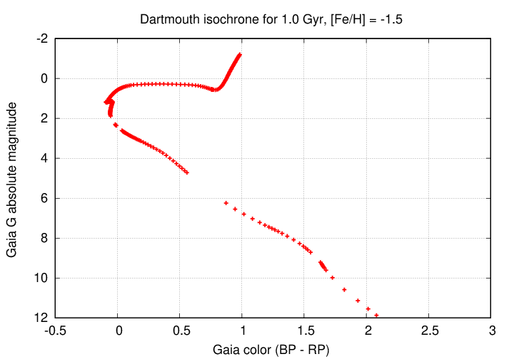
#NUMBER OF AGES= 1 MAGS= 3
#----------------------------------------------------
#MIX-LEN  Y      Z          Zeff        [Fe/H] [a/Fe]
# 1.9380  0.2459 5.4651E-04 5.4651E-04  -1.50   0.00
#----------------------------------------------------
#**PHOTOMETRIC SYSTEM**: Gaia DR2 Revised (Vega)
#----------------------------------------------------
#AGE= 1.000 EEPS=269
#EEP   M/Mo    LogTeff  LogG   LogL/Lo  Gaia_G Gaia_BP Gaia_RP
   3  0.122262  3.5434  5.2856 -2.6334 11.8627 12.9576 10.8758
   4  0.134668  3.5498  5.2395 -2.5197 11.5442 12.5915 10.5768
   5  0.154683  3.5586  5.1880 -2.3729 11.1335 12.1232 10.1913
   6  0.191483  3.5714  5.1358 -2.1768 10.5844 11.5001  9.6769
   7  0.248622  3.5839  5.0790 -1.9566  9.9829 10.8353  9.1076
   8  0.295474  3.5912  5.0433 -1.8166  9.6062 10.4250  8.7489
   9  0.309899  3.5933  5.0293 -1.7737  9.4920 10.3016  8.6397
  10  0.316763  3.5942  5.0210 -1.7523  9.4355 10.2410  8.5854
  11  0.321189  3.5947  5.0149 -1.7378  9.3974 10.2002  8.5487
  12  0.324534  3.5952  5.0096 -1.7263  9.3672 10.1681  8.5196
  13  0.327555  3.5955  5.0045 -1.7157  9.3394 10.1386  8.4928
Columns 7 and 8 contain the "BP" and "RP" magnitudes for the model stars; each line shows the properties of stars with a different mass.
  Q:  Can you make an HR diagram using this datafile?
      Use "G" magnitude on the vertical axis and the
      difference "(BP-RP)" on the horizontal axis.
      Don't forget to put luminous stars at the top!
An example I made is shown below.
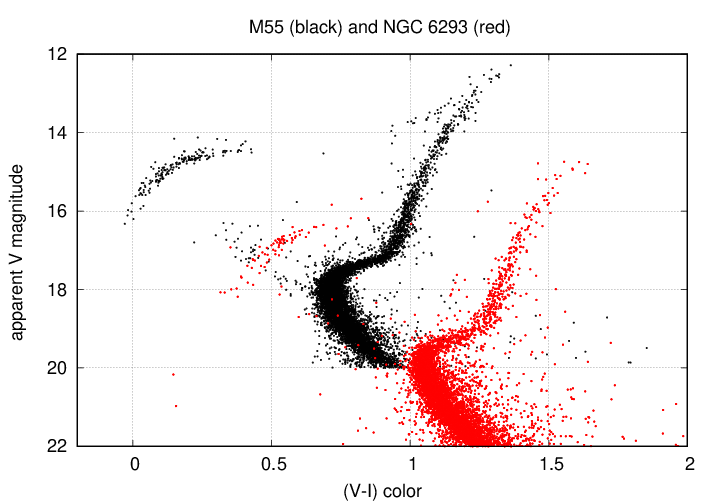
Let's put all this theory into practice. We'll start with one globular cluster, M55, which has a known distance: 5.4 kpc. Suppose we want to measure the distance to the cluster NGC 6293.
Yes, yes, astronomers have measured the distance to this cluster already. Just play along, okay?
Our first job is to create HR diagrams for each of these clusters. Fortunately, both have data in the wonderful Vizier system. You can find the data with a simple search by the cluster name. I've already done that:
In fact, I grabbed the data and edited it a bit, throwing away most of it (and good stuff, too!), leaving just the bits you need to make an HR diagram. Each datafile has a two-column format, with the V-band magnitude in column 1 and the I-band magnitude in column 2, like this:
#RESOURCE=yCat_51322171
#Name: J/AJ/132/2171
#Title: VI photometry of NGC 6293 and NGC 6541 (Lee+, 2006)
#Table J_AJ_132_2171_table3a:
#Name: J/AJ/132/2171/table3a
#Title: Color-magnitude diagram data for NGC 6293
#
#  V      I
17.648 16.194
18.108 16.689
19.499 18.197
19.493 18.397
19.231 17.999
Your job is to do the following:
If you are having trouble, you might want to peek at this graph, or maybe even zoom in on the main-sequence turnoff.
Q: What distance did you determine for NGC 6293?
I have read that the actual distance is about 8.4 kpc. I suspect that your value is quite a bit larger.
  Q:  Can you think of any effect that we might have ignored
      in our calculation?
Yes! That's right. Extinction! The values in these catalogs are observed magnitudes, not corrected for extinction due to dust and gas along the line of sight.
When light passes through clouds of gas and dust, some of the photons interact with the atoms and particles, bouncing off in new directions. This scattering of light causes two effects in the light which passes through the cloud and reaches the other side:
But also, because short-wavelength light is scattered more efficiently than long-wavelength light,
You should all recognize these effects, as you see them nearly every day as the Sun moves from nearly overhead

to low on the horizon at sunset.

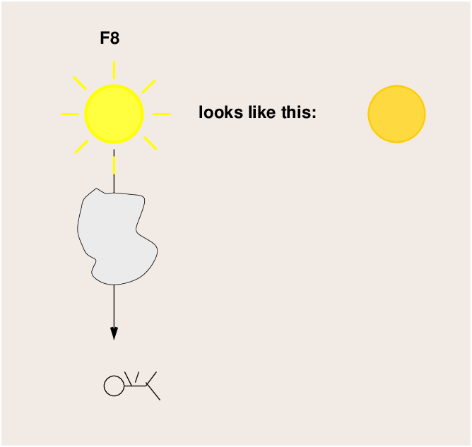
This is true of light passing through the Earth's atmosphere, and also of light passing through the interstellar medium. Clouds of gas and dust between a star and the Earth can lead to exactly the same two effects. A bright, yellow star, for example, may end up looking dim and orange.
Fortunately, there is a way that astronomers can detect these effects, and even -- to some extent -- correct our measurements. The key is that, under most circumstances, there's a simple connection between reddening (change in COLOR) and extinction (change in BRIGHTNESS). If we can measure the change in color, we can correct the magnitudes to remove the extinction. For example,
A(V) = 3.1 * E(B-V)
The numerical factor connecting reddening to extinction changes a bit, depending on which filters are used to measure the magnitude and color of a star. You can look up some common values in textbooks or websites on astronomical photometry; several are listed in this lecture from AST 613.
In the case of our two globular clusters, it's obvious that there's a difference in the color of the main-sequence turnoff locations.
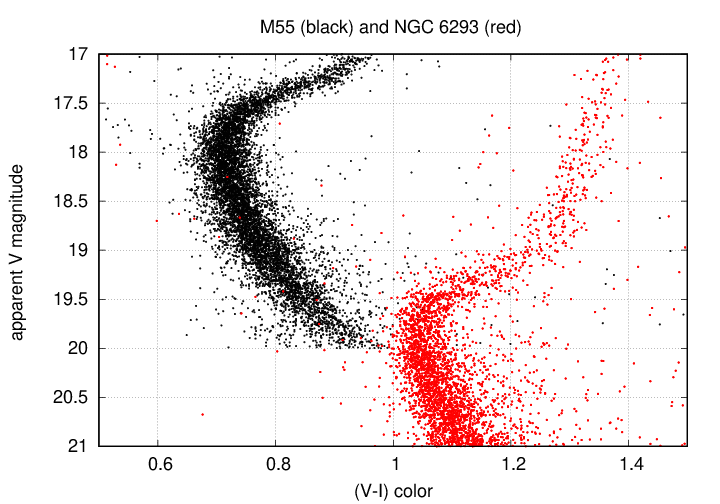
  Q:  If the stars in these two clusters ought to have identical colors,
          by how much as NGC 6293 been reddened?  In other words,
          by how many magnitudes has its color been shifted to the right?
Astronomers have determined empirically relationships between the amount by which stars have been REDDENED, and the amount by which they have been EXTINGUISHED (made fainter). The values depend on which filters one uses to make the measurements, but in this case, for every magnitude of reddening in (V-I) suffered by a star, it has been made fainter by about 2.6 magnitudes in the V-band. We can use this relationship to "de-redden" the measurements of all the stars in NGC 6293.
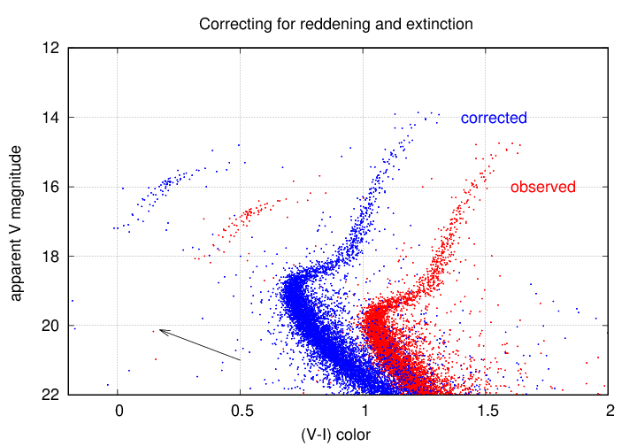
Having corrected the measurements of stars in NGC 6293, we can try a second time to determine its distance relative to the nearby M55.

  Q:  What is the difference in V-band magnitude
      for the main-sequence turnoff now?


  Q:  Recall that M55 is at a distance of 5.4 kpc.
      Compute a new distance for NGC 6293 based on this
      corrected color-magnitude diagram.  What is it?


      How does it compare to the literature
      value of 8.4 kpc?
In order to tie the RELATIVE distances of clusters to an ABSOLUTE scale, we need to know the real distances to some nearby star clusters via parallax. Back in the "old days", this was not so easy. Astronomers spent many years working on a few nearby clusters, trying very hard to avoid systematic errors and cross-check their results.
Two of the most commonly used nearby clusters are the Hyades and the Pleiades, both relatively young open clusters, both visible to the naked eye in the winter sky. We can see our estimates of the distance to the Hyades have not changed (much) over the last few decades:
 year    method           distance              reference
-----------------------------------------------------------------

 1967    parallax,
         emission lines,
         convergence,      48.3                Hodge and Wallerstein, PASP 78, 411 (1966)

 1967    revised           44.3                Wallerstein and Hodge, ApJ 150, 951 (1967)


 1997    FGS parallax      46.1                van Altena et al., ApJ 486, L123 (1997)

 1997    binary star       47.4  +/- 2.3       Torres et al., ApJ 479, 28 (1997)

 1998    Hip parallax      46.34 +/- 0.27      Perryman et al., A&A 331, 81 (1998)

 2017    Gaia parallax     46.75 +/- 0.46      Gaia Collab, A&A 601, A19 (2017)


-----------------------------------------------------------------
The most recent paper in that table , published just a few months ago, presents analysis of the distances to 19 open clusters, including the Hyades and Pleiades. We can now make accurate HR diagrams for a number of clusters, allowing us to use them for relative distance measurements, AND allowing us to check our models of stellar evolution.
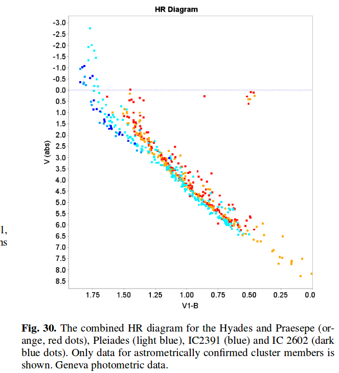
Figure 30 from
Gaia Collab, A&A 601, 19 (2017)
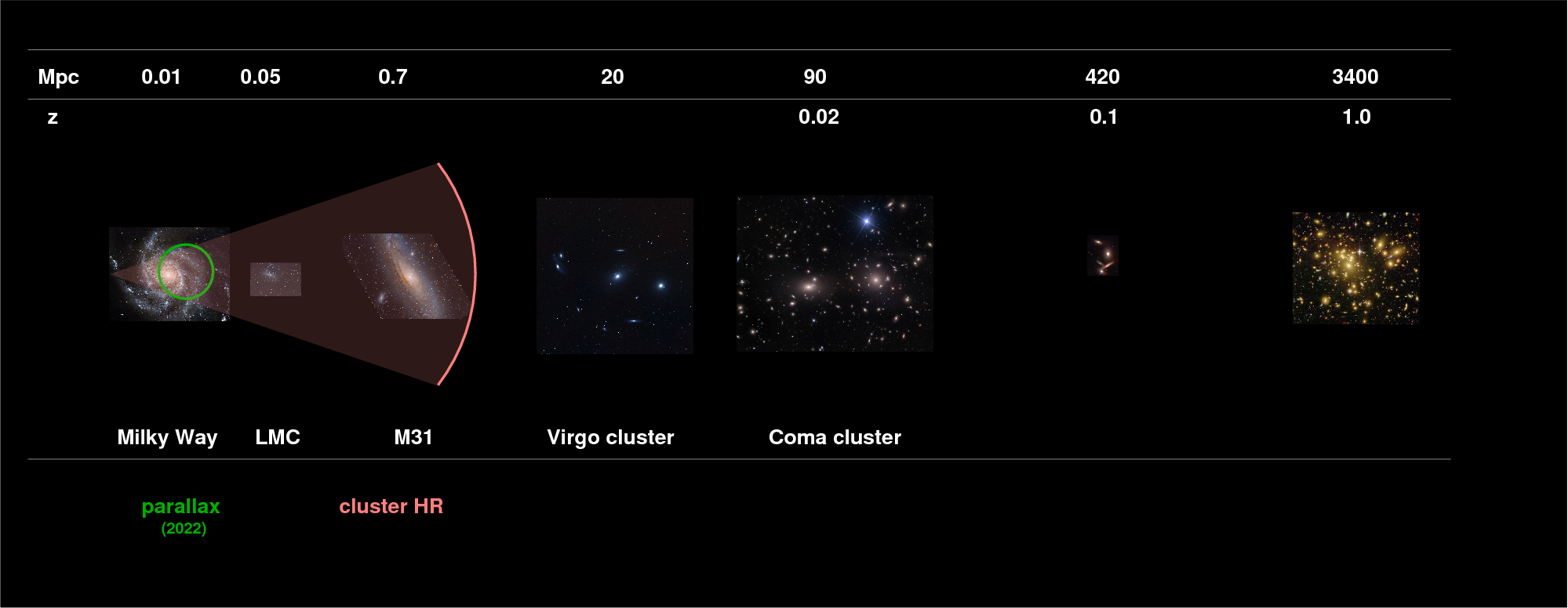
The answer is -- pretty far! We can easily measure the color-magnitude diagrams of open and globular clusters in our own Galaxy, even with ground-based telescopes. Using space telescopes such as HST and JWST, we can even make out the properties of individual stars in clusters in some other Local Group galaxies.
For example, the Small Magellanic Cloud (SMC for short) is one of the Milky Way's satellites, and one of our closest galactic neighbors.

Image of Magellanic Clouds and the Paranal Observatory
courtesy of
Y. Beletsky/ LCO/ESO.
One can find many young star clusters within the SMC, including this one, known as NGC 419. The authors of The Search for Multiple Populations in Magellanic Cloud Clusters III: No evidence for Multiple Populations in the SMC cluster NGC 419 suggest that this cluster has an age of 1.4 Gyr and a metallicity of about [Fe/H] = -0.7.

Figure 2, left panel,
taken from
Martocchia et al., MNRAS 468, 3150 (2017)
   Q:  Generate an isochone with age 1.4 Gyr and [Fe/H] = -0.7,
       and compare it to this color-magnitude diagram of NGC 419.
       (Or just grab this CSV datafile., using col 3 for x-axis, col 1 for y-axis)

       What is the absolute G magnitude (same as mF814W) of stars at the main-sequence
       turnoff for the model stars?

       What is the apparent mF814W magnitude of stars at the main-sequence
       turnoff for NGC 419?

       What is the distance to the SMC based on this cluster?
But we can extend our measurements well beyond the Magellanic Clouds. In recent years, some astronomers have used HST (and soon will use JWST) to investigate properties of stellar clusters in the Andromeda Galaxy. See, for example, Davis et al., ApJ 884, 115 (2019). Even the best images barely resolve the individual stars ...
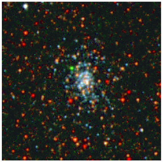
Figure 1 taken from
Davis et al., ApJ 884, 115 (2019)
... but a color-magnitude diagram does (after some judicious pruning) reveal members of an open cluster.

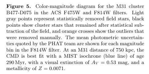
Figure 2 taken from
Davis et al., ApJ 884, 115 (2019)
   Q:  Generate an isochone with age 0.29 Gyr and [Fe/H] = +0.01,
       and compare it to this color-magnitude diagram.
       (Or just grab  this CSV datafile  and plot col 3 on x-axis, col 1 on y-axis)

       What is the absolute mF814W magnitude of the main-sequence turnoff point in the models?

       What is the apparent mF814W magnitude of the main-sequence turnoff point in the observed cluster?

       What is the distance to the M31 based on this cluster?
So, using clusters of stars, we can finally escape the Milky Way and begin to measure distances to the extragalactic universe.
Copyright © Michael Richmond.
This work is licensed under a Creative Commons License.