 Copyright © Michael Richmond.
This work is licensed under a Creative Commons License.
Copyright © Michael Richmond.
This work is licensed under a Creative Commons License.
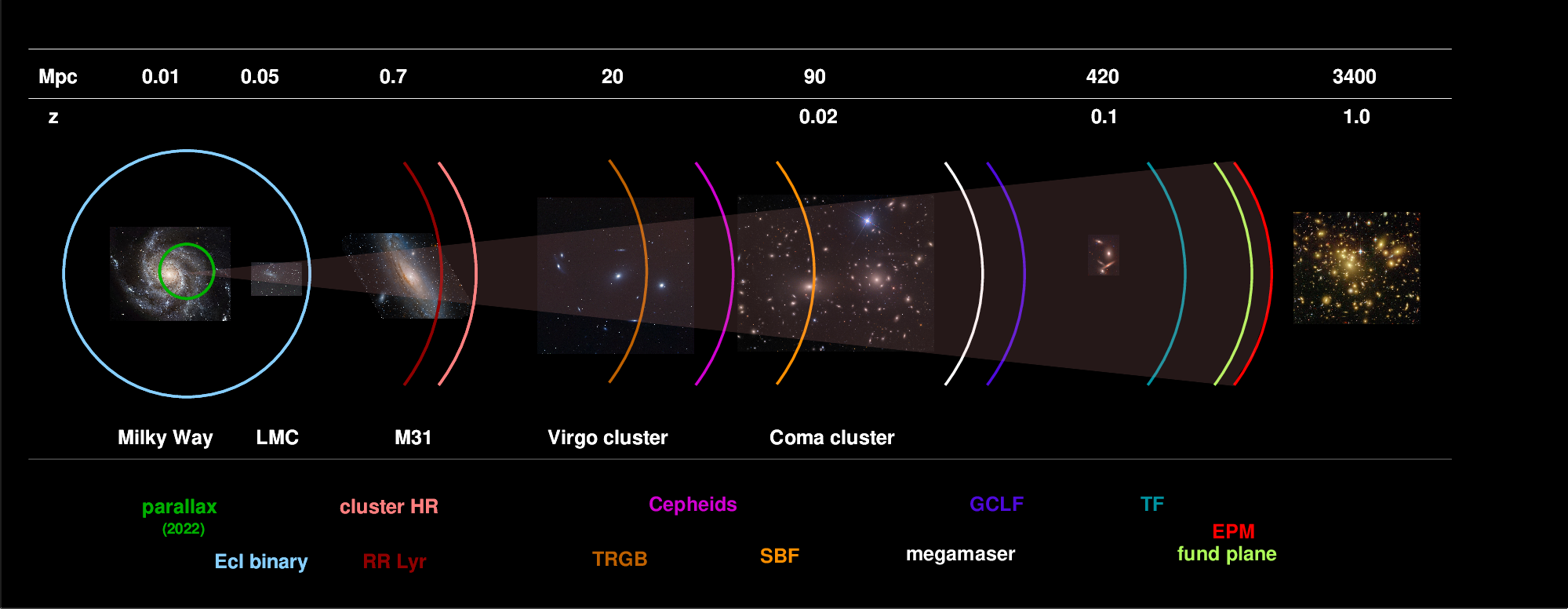
The methods we've described so far can only reach out to the nearest galaxy clusters. If we wish to probe deeper into the universe, we need to find new ways to estimate distances. Because supernovae are very, very, VERY luminous events, we can see them at large distances ... but can we find a way to use them to measure those distances?
The topic is a big one, so I'll split it into two lectures. Today, we'll look at supernovae in general, and then focus on a variety called "Type II". Next time, we'll concentrate on a different type of stellar explosion, the "Type Ia" supernovae.
The short answer is "a star which explodes."
Now, there are several mechanisms which cause a star to explode, and the pre-explosion object can have several different forms. We'll discuss some of those issues a bit later.
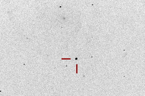
But from an observational point of view, a supernova is a star which suddenly appears in a galaxy, shines as brightly as an entire galaxy for a few weeks or months, and then gradually fades away. Here are a few nice examples of recent supernovae.
SN 2011 in M101
Images of SN 2011fe in M101 courtesy of
PTF and B. J. Fulton
SN 2014J in M82

Images of SN 2014J in M82 courtesy of
Scott McNeil
SN 2017eaw in NGC 6946.
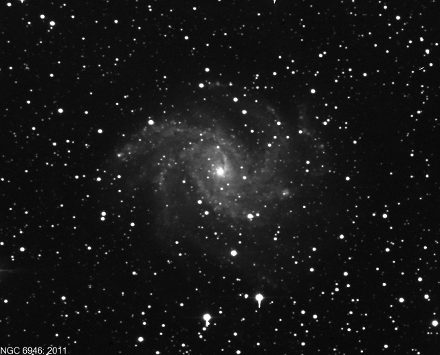
Image of SN 2017eaw in NGC 6946 courtesy of
Gianluca Masi and the Virtual Telescope Project
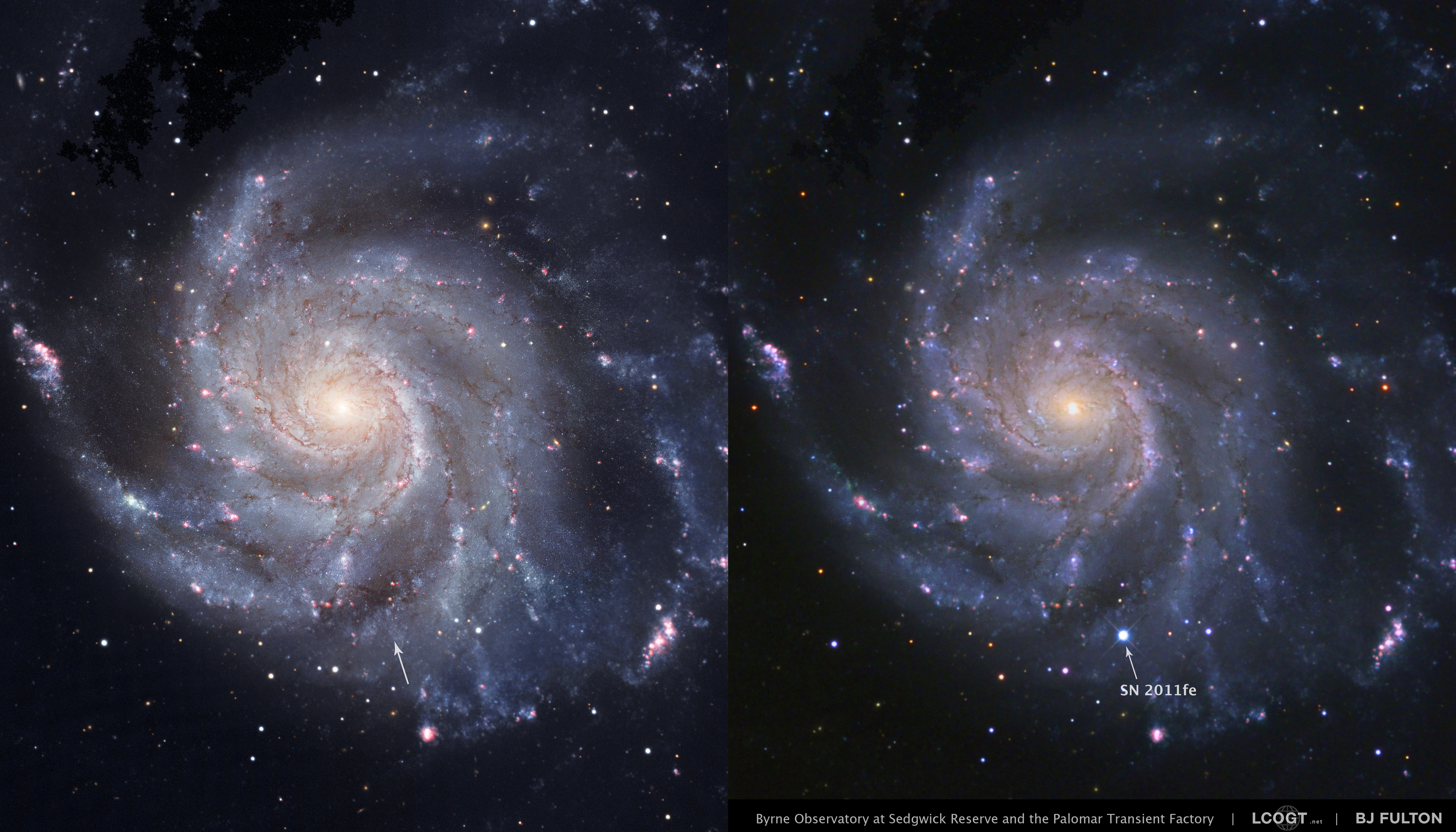
Now, these pictures don't really show how bright a supernova can be. In many cases, a supernova can outshine all the stars in its host galaxy for a brief period. For example, the earlier pictures of SN 2011fe in M101 give the impression that the SN was just one little blob of light among many others ...
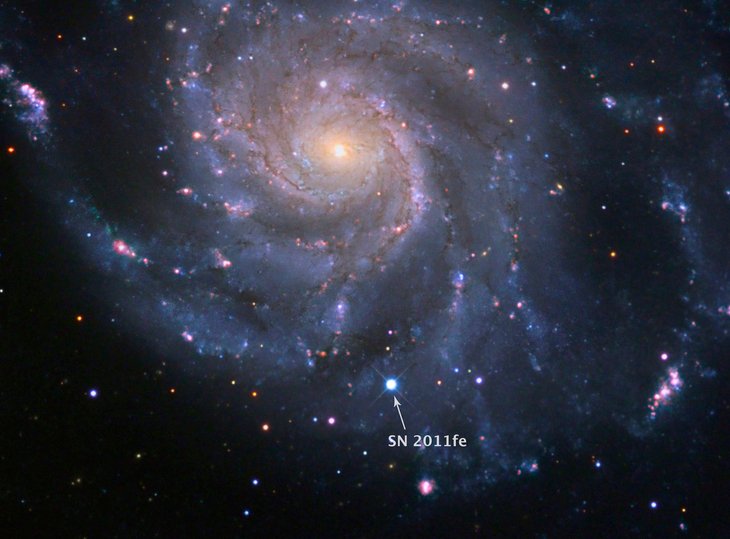
Image of SN 2011fe in M101 courtesy of
PTF and B. J. Fulton
and cropped by me.
But if one uses a little telescope, like my 12-inch Meade LX200 at the RIT Observatory, and takes only a short exposure, then we can compare the light from the galaxy's nucleus and spiral arms to that from the supernova more clearly. Below is an R-band (red light) image taken on Sep 25, 2011, when SN 2011fe was already past its peak brightness and starting to fade.
R-band image of SN 2011fe in M101 courtesy of
Michael Richmond and the RIT Observatory
And below is an image taken through a B-band (blue light) filter. The SN, all by itself, produces much, much more blue light than the billions of stars in the nucleus of this galaxy!
B-band image of SN 2011fe in M101 courtesy of
Michael Richmond and the RIT Observatory
This is even worse because SNe ...
The star "S Andromeda" was a type Ia explosion in the Andromeda Galaxy, but it happened just a few decades before astronomers were ready with equipment powerful enough to study it properly.
Thirty years ago, in 1987, a supernova appeared in the Large Magellanic Cloud. It was close enough that neutrinos from the explosion were detected on Earth, but no event since then has even come close.
There is a very wide variety of supernova classes and sub-classes. It's easy to get lost in the different types and designations. For our purposes, all those fine distinctions aren't necessary. Even though there APPEAR to be many different types, one can in the end separate them into just two varieties.
Want some practice? Look at the following pictures, and try to separate the four different animals into two species. All the individuals pictured have two legs, one head, and stand about two meters tall.
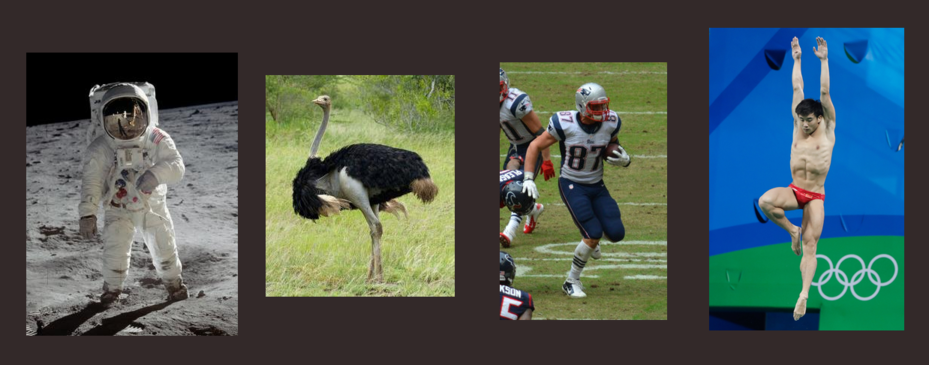
Image of ostrich courtesy of
berniedup and Wikipedia .
Image of Rob Gronkowski courtesy of
Wellslogan and Wikipedia.
Image of Apollo astronaut courtesy of
NASA.
Image of Cao Yuan courtesy of
Fernando Frazão/Agência Brasil and Wikipedia
(I hope you got this right)
There are just TWO species, even though all the pictures look quite different.
         Human                             Ostrich
  --------------------------------------------------------------
    hidden behind many layers of         covered by feathers
        spacesuit

    hidden under an NFL uniform
        and helmet

    not covered by clothing
  --------------------------------------------------------------
The three different humans LOOK different because they are wearing different amounts of material over their bodies; if you could slice each human in half, you'd find the same stuff inside: bone, muscle, blood, etc.
Well, it's the same thing with supernovae. There are just two varieties, really, but one of them wears quite a range of clothing.
        Massive Star Core                  White Dwarf
  --------------------------------------------------------------
     Type IIP  - hidden under thick            Type Ia
        envelope of hydrogen

     Type IIb  - hidden under a thin
        layer of hydrogen, covering
        thin envelope of helium

     Type Ib   - hidden under thin
        envelope of helium

     Type Ic   - hidden under a
        thin envelope of C, O, etc.
  --------------------------------------------------------------
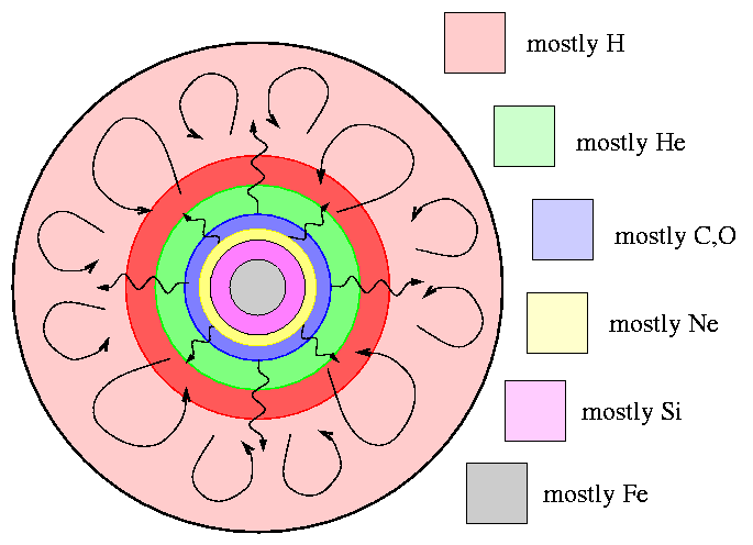
arise because the
core of a massive star (at least 8 solar masses
when born) has fused its way through all the
hydrogen, helium, carbon, oxygen and other
materials, ending up with a bunch of iron-group
elements at its center.
Iron nuclei do not release energy when they fuse --
instead, they absorb it from their
surroundings.
So, to be brief, when the core reaches this state,
it cannot generate energy to maintain the thermal
pressure which counteracts gravity;
and so, the core collapses.
The exact mechanism is very complicated
and hundreds of other papers ...
but the end result is
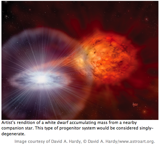
arise from binary-star systems in which an ordinary
main sequence star is close to a carbon-oxygen white dwarf
(the single degenerate scenario).
Material from the main-sequence star can -- under the right
circumstances -- escape from the outer atmosphere
and form an accretion disk around the white dwarf.
If the rate of mass accretion onto the white dwarf falls
into the proper range,
then the white dwarf's mass may eventually reach
the Chandrasekhar limit, about 1.4 solar masses.
At that point, little regions of thermonuclear reactions near the
center of the white dwarf may enter a runaway
instability,
turning most of the white dwarf from C-O to Fe-group
elements and producing enough energy to blow the entire
star out into space.
Well, that's one possibility. Another is that TWO white dwarfs in a close orbit may eventually merge (the double degenerate scenario). The merger creates a single object which again exceeds the Chandrasekhar limit, and, once again, Ka-Boom.
In this case,
In both cases, very roughly 1051 ergs = 1044 Joules of energy are released by the, um, complex processes occuring within the central regions of the progenitor star.
  Q:  The Sun's luminosity is L⊙ = 4 x 1026 Joules/sec.
         How long would the Sun have to shine to release as much energy
         as a supernova explosion?
So, to a very very rough approximation, in both cases, we see the same thing: an expanding cloud of extremely hot gas, flying outward at very high speeds, reaching absolute magnitudes of Mv ~ -17 to Mv ~ -21.
How can we use this big explosion to measure a distance?
For measuring distances, we will concentrate on just one of the sub-types of the "Massive Star Core" supernovae. A Type IIP event involves the core collapse inside a star which still retains most of its massive envelope of hydrogen. In very simple terms, when the core collapses,
The shock wave heats the bulk of the star and accelerates it outward, to speeds far above the escape velocity. In a word, the star explodes. However, if one looks more closely, one finds that the velocities of different layers of the star vary in a systematic way: material from the inner regions has a relatively small velocity, while material from the outer regions has a relatively high velocity. We call this homologous expansion. (Click on figure below to animate)
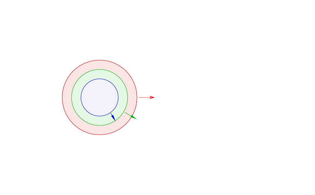
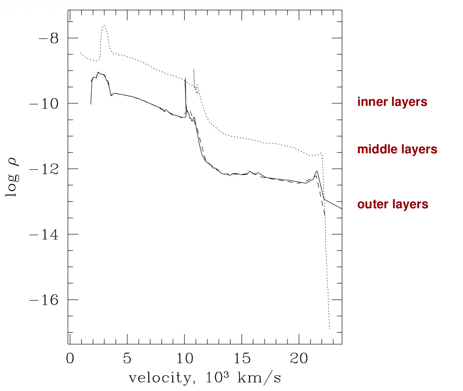
Figure modified from
Blinnikov et al., ApJ 496, 454 (1998)
The shock wave heats material up to very high temperatures, well over 100,000 Kelvin, ionizing all the hydrogen. The outermost layers emit X-rays and UV for several hours after the shock breaks out of the star, but then cool off quickly. When the temperature of the gas falls to roughly 6000 Kelvin, however, the hydrogen begins to recombine. At this point, as the outermost layer switches from ionized to neutral, its opacity drops: neutral hydrogen gas is MUCH more transparent than ionized gas.
When the outermost layer recombines, it becomes essentially transparent, and we can see into the layer below it. This layer is still hot enough that hydrogen is ionized ... but within a short time, it, too, cools off to about 6000 Kelvin and recombines. When it becomes transparent, we can then see into the NEXT layer of the star, and so on and so on.
The important facts here are
As time goes by, and we see further into the star, the velocity of this special layer will decrease. The graph below shows the evolution of a computer model of a Type II supernova -- the lines are drawn at roughly one-week intervals.

Figure taken from
Kasen and Woosley, ApJ 703, 2205 (2009)
The solid curve in the figure below shows the evolution of a computer model of an exploding star, while the circles show measurements of real supernovae.

Figure taken from
Kasen and Woosley, ApJ 703, 2205 (2009)
The radius of any particular layer of material at some time t can be written as

where t0 is the time of explosion and R0 is the radius of that layer at the time of explosion. With high-quality spectra of the supernova, we can measure the velocity of of one particular layer of the star -- the layer which happens to be acting as the photosphere at the moment.
Because the photosphere is in such a simple condition -- nearly pure hydrogen, at a temperature close to 6000 K -- it isn't too difficult to compute the radiation it emits. To first order, the photosphere acts like a "dilute blackbody", emitting luminosity
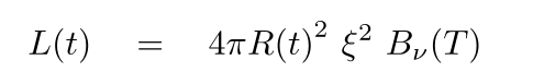
where T is the temperature ~ 6000 K, and ξ is a "dilution factor", inserted into the ordinary blackbody equation to account for several factors which cause the spectrum of the actual star to differ from that of a perfect blackbody.
Using spectroscopy and photometry, we can measure v(t) and the observed flux f(t). If we make measurements at several different times, when the photosphere has different sizes and luminosities, we have enough information to solve for the time of explosion, initial size of the star, and determine the distance as well; it's just a matter of comparing the luminosity L(t) to the observed flux f(t) and using the inverse square law (and hoping that there was no extinction, etc.).
It is a nice coincidence that the speed with which the recombination wave runs deeper into the star is very roughly the same as the rate at which the star is expanding; in other words, the radius of the apparent photosphere doesn't change a great deal while the wave is still moving through the envelope. As a result, the luminosity of Type IIP supernovae hits a plateau (hence the "P") and remains nearly constant for a month or two.
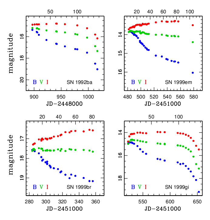
Figure taken from
Jones and Hamuy, RMxAC, 35, 310 (2009)
On July 26, 2013, astronomers noticed a bright new star in a rather photogenic spiral galaxy known as M74. (Click on the image below to see before/after animation)

Image courtesy of
Capella Observatory and Makis Palaiologou, Stefan Binnewies, Josef Popsel
I (and many other astronomers) monitored the brightness of this supernova over the next few months. Its light curves show clear evidence for a "plateau" as the photosphere recedes into the ejecta. Let's use this nearby SN IIP 2013ej in M74 to illustrate the method by which astronomers to measure the distance to a supernova.

Figure 3 of
Richmond, JAVSO 42, 333 (2014)
We'll use only the V-band measurements for this quick little in-class calculation. Let's pick the date JD = 2456510, which is just a bit after the time of maximum light.
  Q:  Step 1: What is the apparent V-band magnitude of
        this SN on the date 2,456,510?

Taken from Figure 3 of
Richmond, JAVSO 42, 333 (2014)
This apparent magnitude can be converted to a flux of optical light measured by our telescopes. In this particular case, for an apparent magnitude of mV = 12.5, the flux turns out to be

If one assumes that the photosphere is emitting like a blackbody, then one can estimate the temperature by fitting the measured fluxes to spectra of Planck functions for different temperatures. The temperature will decrease with time, in general.
  Q:  Step 2: What is the temperature of the photosphere of
        this SN on the date 2,456,510?
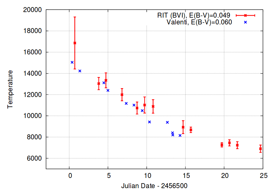
Taken from Figure 8 of
Richmond, JAVSO 42, 333 (2014)
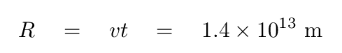
Spectra of this event showed that at this time, 16 days after the explosion, the photosphere had a velocity of about v = 10,000 km/s = 107 m/s. If we assume that this layer of gas has been expanding into space at a constant speed for the past 16 days, then we can easily compute the radius of this glowing layer of hot gas.
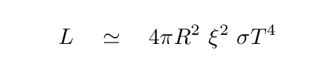
If we pretend that the expanding cloud of gas emits radiation just as a diluted blackbody would, then we can calculate the luminosity of the supernova at this moment; well, we need to know the value of the dilution factor ξ. A very rough value might be ξ = 0.2.
Let's review:
  Q:  Given all this information, how can we derive the distance
           to the supernova?
Yes, exactly: by comparing the APPARENT magnitude to the ABSOLUTE magnitude,
or by comparing the LUMINOSITY to the FLUX,

we can find at least an approximate value for the distance d to the supernova.
  Q:  Use our estimated values for R, T, and ξ
           to compute the luminosity L of this SN at day 16.

                L  =  ___________


  Q:  Then use this luminosity and the observed flux f to compute
           the distance to the supernova.

                                  L
                d  =   sqrt( -------------- )
                                4 π f
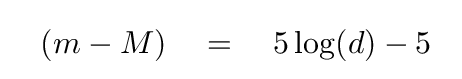
When I went through a somewhat more complicated version of this procedure, using data for this supernova, I found that the Expanding Photosphere Method yielded a distance of about 9.1 +/- 0.4 Mpc. How well does that agree with distances determined by other astronomers, and using different methods?
EPM has some weaknesses and strengths:
We can apply this technique to large distances, because Type IIP SNe are very luminous: their typical absolute magntiudes are between -15 and -18.
Figure 7 taken from
Gall et al., A&A 611, 25 (2018)
Copyright © Michael Richmond.
This work is licensed under a Creative Commons License.
_male_(13994461256).jpg)