 Copyright © Michael Richmond.
This work is licensed under a Creative Commons License.
Copyright © Michael Richmond.
This work is licensed under a Creative Commons License.
Today we address one more aspect of the CMB, then move on to ask "What happens to the universe -- will it keep expanding forever?"
Back in the early universe, space was filled with very hot, very dense gas. Suppose we look at some region where the gas properties are pretty much average. A cloud of gas from a neighboring region approaches our gas, moving to the right.
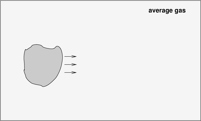
The motion of the cloud pushes on the gas in our region, causing it to pile up in front of the cloud. The gas there is shoved together into a region of slightly higher density and pressure.
Now, this region of slightly higher pressure pushes against the undisturbed gas to its right, compressing IT and causing IT to have a higher density and pressure.

This disturbance continues to move through our region, creating little areas in which the density and pressure are higher than average.

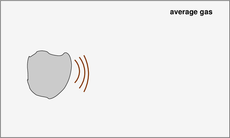
  Q:  Is there another name of "a disturbance, characterized by regions of
             higher pressure and density, which moves through a fluid?"
Yes! This is also called a "sound wave." The region of higher pressure propagates through space with a velocity vs often called "the speed of sound." This speed depends on the properties of the gas. During the early universe, when the average gas density was very high, the sound speed was very fast.

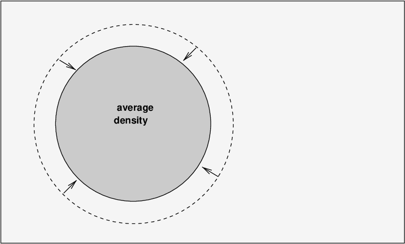
Consider a little region of gas in the early universe -- at some time between t = 3 minutes and t = 300,000 years. Suppose that, by some random set of collisions and motions, this region at some moment happens to end up with a slightly higher-than-average density.

The gravitational force of the clump will pull gas from the surrounding region inwards, increasing the density of the clump.
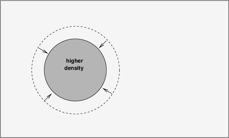
However, as the clump shrinks, the density and temperature of the gas inside rises. Recall that, in addition to the MATTER inside this clump -- protons and electrons and neutrons -- there are a bunch of PHOTONS trapped within it as well. At this point in the evolution of the universe, the electrons are running free of the nuclei, the gas is fully ionized, and as a result, it is opaque. Photons can't escape from the clump, so they are pressed closer together as it shrinks. The radiation pressure from the photons helps to push back against this contraction.
Eventually, after reaching a minimum size, the clump stops collapsing and begins expanding again. It grows larger, reaching its initial size ...
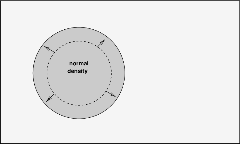
... but then the momentum of the expansion causes the gas to overshoot, and the cloud grows even larger than it was originally.

Of course, now the cloud is LESS dense than the surrounding gas, and has a lower pressure as well. The pressure of the material around halts the expansion and causes it to contract again ...
... but, again, it overshoots the original size and starts shrinking again.
To summarize, small random variations in density in the early universe can set up regions in which the gas oscillates in and out, growing and shrinking, for long periods of time.
The outer edges of the clump expand and contract by pushing outward against the ambient gas, then being pushed back inward. The boundary between clump and ambient gas moves at the speed of sound vs, and so this phenomenon is often called acoustic oscillations.
How big are these clumps? There are many different sizes -- big ones, small ones, intermediate ones. The one thing they share is the speed with which their boundaries move: all of them expand and contract at the speed of sound.
This oscillation is driven in part by the pressure exerted by particles inside the clumps -- and photons play a very important role in resisting the compression of the clumps.
Q: What happens to the photons at t = 300,000 years after the Big Bang?
Exactly. At the time of decoupling, electrons combine with nuclei to form neutral gas, which is transparent to photons. All of a sudden, photons are free to fly away from their local clumps of gas. When they leave, they remove a large portion of the pressure which was preventing clouds from collapsing. As a result, these acoustic oscillations stop at this time.
When the photons leave a clump, they carry with them a bit of information about the gas within that clump. The temperature in a dense clump is higher than the average value, so the photons leaving a dense clump have a slightly higher energy than average. Likewise, the photons streaming out of a region of low density will have slightly lower energies than average. These small differences in energy remain unchanged as the photons fly through universe, for billions and billions of years ... until our telescopes collect them.

Image taken from
Mallaby-Kay et al., ApJS 255, 11 (2021)
Now, which regions will produce the most obvious variations in the CMB? That is, what sort of region in the early universe will produce either particularly high-energy ("hot") or low-energy ("cold") photons? Clearly, the most extreme variations in CMB temperature will come from the clumps which have extreme variations in density. Let's examine such clouds more carefully.

We've picked two special clouds. The cloud on the left has reached its maximum outward expansion, having grown by a distance d, and is just about to start contracting. The cloud on the right has contracted to its minimum size, having shrunk by the same distance d, and is just about to start expanding again. Why are these two clouds special? Because they have been changing continuously in just one direction -- expanding (on left) or contracting (on right) -- for the entire duration between the end of nucleosynthesis and the moment of decoupling.
In other words, these two clouds have changed in size by a distance

This is the maximum distance by which a clump could expand -- or shrink -- during this long, long period between the Big Bang and the moment of decoupling. This maximum distance d is sometimes called the "fundamental scale" of the universe at the moment of decoupling. Since clumps which had expanded or contracted by this amount ought to have been at the very peak of either high or low density, we expect that we ought to see features of this size prominently when we look at the cosmic microwave background. Of course, from our point of view, far, far, away, we can't measure the distance d directly. Instead, we expect to see many bright (hot) and dim (cool) features in the CMB which are separated by some angle on the sky which corresponds to this distance.
Is there any mathematical way to look for particular separations between features in the CMB? Sure -- there are many techniques for doing so. For example, one could take the Fourier transform of the two-dimensional map of the CMB intensity. However, describing Fourier analysis would take a bit of time ... so let me instead describe very briefly a second method: the two-point correlation function. The basic idea sounds pretty simple:
Given a random CMB spot in a location, the correlation function describes the probability that another spot will be found within a given distance.
How can one measure this probability of finding another spot at some given distance away from a given spot? Well, one method is to start with a map of spots, divide them up in pairs -- all possible pairs! -- and measure the distances between them. The number of pairs with any given separation is a measure of the probability that one will find a second spot at that distance from a first spot. It's a lot easier to understand if you just watch someone do it. Click on the picture below to start a brief animation.
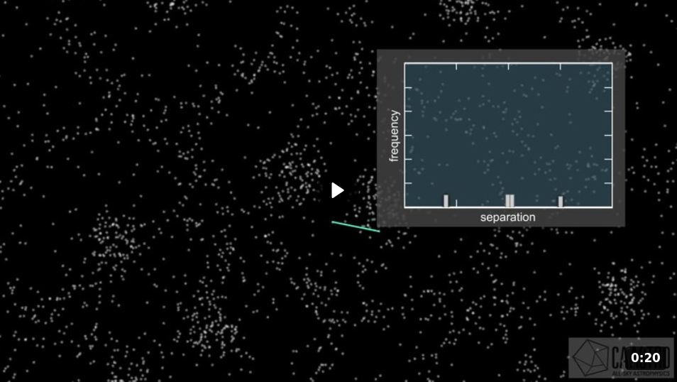
Image and animation courtesy of
Wikimedia and Arc Centre of Excellence for All-Sky Astrophysics
After the Planck satellite finished its four-year mission, scientists used its map of the CMB fluctuations
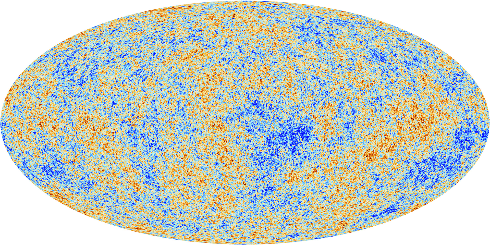
Image courtesy of
ESA and the Planck Collaboration
to compute the power spectrum via Fourier analysis (which is very much like the two-point correlation function). In the graph below, the vertical scale shows the probability that one will find another feature at some given distance from a chosen location.

Image courtesy of
ESA and the Planck Collaboration
The big peak in the power spectrum at an angular separation of about 1 degree corresponds to the "fundamental scale" of clumps of gas in the very early universe. The angular size of this feature -- and the smaller second and third peaks -- allow cosmologists to glean additional information about conditions in the gas way back then.
You do a simple check on this yourself. Look again at this tiny closeup of the CMB, in one small area.
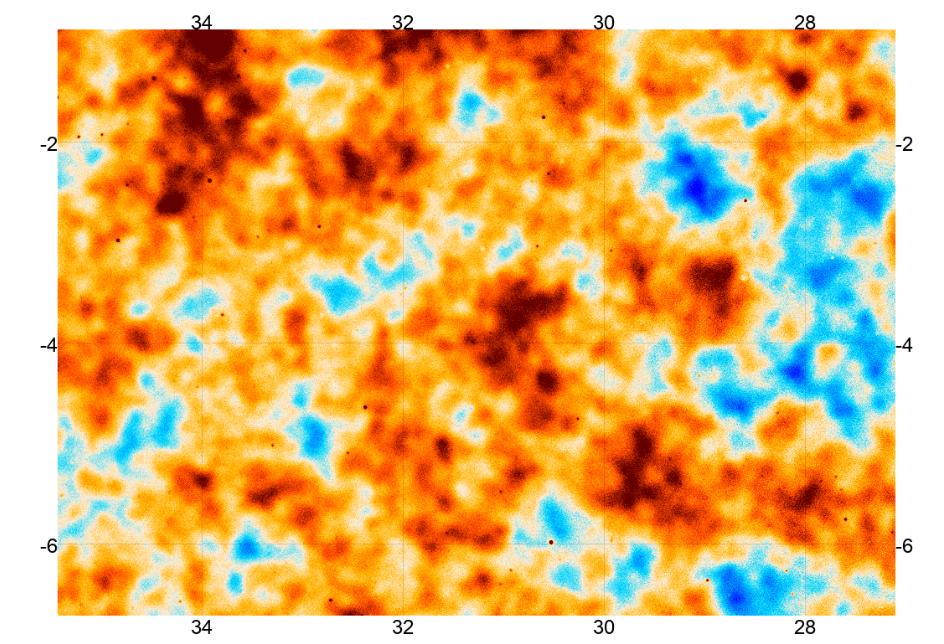
Image taken from
Mallaby-Kay et al., ApJS 255, 11 (2021)
  Q:  What is the typical separation of the features you see
           in this map?


  Q:  How does that compare to the peak of the power spectrum?
We'll assume in the discussion below that the universe contains only ordinary matter; no dark matter, no cosmological constant. This overly simplified model makes it relatively easy to figure out the basic nature of the universe's evolution.
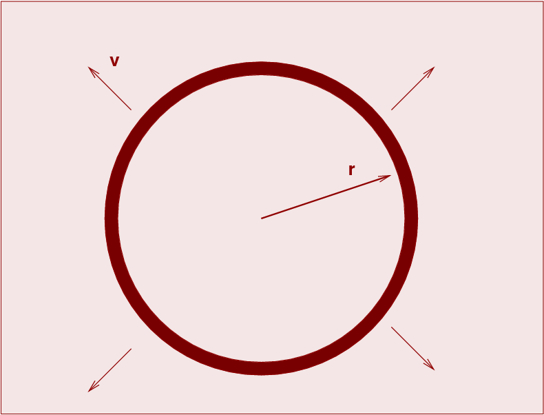
Imagine that the universe is homogeneous and uniform, filled with matter which has the same density everywhere. Let's write the density of material as ρ(t), so at the current time, it has value ρ(t0), Consider a spherical shell of material of radius r, which is currently expanding at velocity v.
What will happen to the shell as time progresses? As you consider this question, remember one of the (many) things Isaac Newton figured out about gravitational forces:
The gravitational forces of a uniform material OUTSIDE a spherical region cancel each other out; the only forces experienced by a shell are due to the material INSIDE the shell.
The answer isn't too hard to figure out. One can make a close analogy to the motion of a cannonball which is fired vertically upward from the Earth's surface. There are two possibilities from a practical standpoint, or three if one is a mathematician.
The same is true for this shell of material. Let us demonstrate.
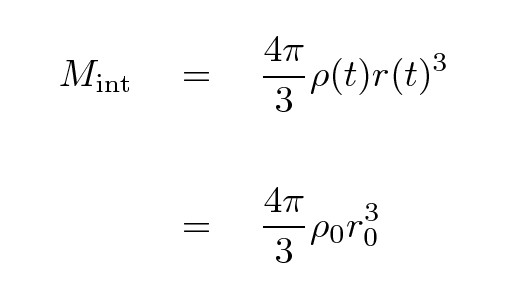
As mentioned a moment ago, because the material OUTSIDE the sphere is uniform, we can ignore the gravitational forces from all the material outside the shell. That means that the dynamics of the shell depend only on the total mass enclosed by it. We will assume that the peculiar motions of matter are so small, compared to the large-scale motion of the shell as a whole, that the interior mass doesn't change as the shell expands.
The shell itself has some mass m. We can write the total energy of the shell as a sum of its kinetic and gravitational potential energies. For reasons which will become clear later, I'll write that total energy in one particular manner.
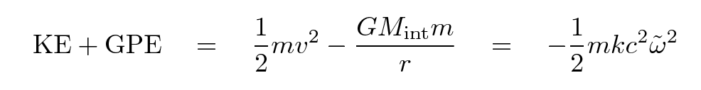
Now, as mentioned in the previous lecture, astronomers break the distance to an object into a portion which doesn't change with expansion, called the "comoving coordinate" and denoted as an ω with a tilde over it, and a portion which does, called the "scale factor" and written as a(t). If we substitute
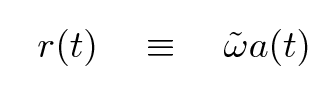
where

and do a little simplification, we end up with
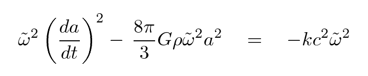
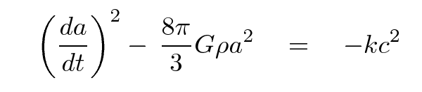
Let's stop for a moment and look at the result. The left-hand side shows the two terms which add up to form the total mechanical energy (per unit mass) of our shell of matter, and so the right-hand side must also be proportional to that energy. What are the possibilities?
It certainly would be nice to figure out the fate of our universe. Let's see if there is some way to convert that expression into one which contains observable quantities.
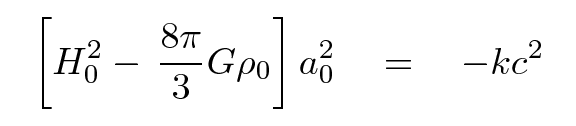
You may recall from the previous lecture that the Hubble parameter H(t) is related to the scale factor a(t) and its rate of change.

If we substitute this expression into our previous "energy equation", we end up with

Now, this equation is valid for any choice of time. Note that the right-hand side isn't changing at all -- all the action is in the terms on the left. If we can measure some values which appear on the left hand side at ANY choice of time, we can compute the value of the right hand side once and for all. That, in turn, will tell us the fate of the universe.
So, what's a good time to choose? How about .... RIGHT NOW! I'll use a shorthand for t = now by placing a zero subscript on quantities; that turns H(t) into H0, which may look familiar to you.
  Q:  What is the value of H0?


  Q:  Can you compute the value of the
      critical density of the universe at
      the current time?  (Recall G = 6.67 x 10⁻¹¹ N*m2/kg2)
The critical density is an important value, but if one specifies it in grams per cc or kg per meter cubed or atoms per cubic meter, it always seems to involve a large negative exponent. For convenience, cosmologists often discuss the matter density in a relative way:
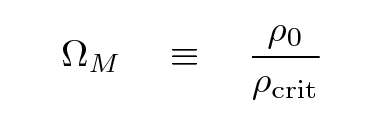
The "M" subscript refers to all matter, ordinary baryonic and exotic dark matter alike.
What is the value of ΩM? There are many ways to measure it. Below are some values from a review published in 2002 ...
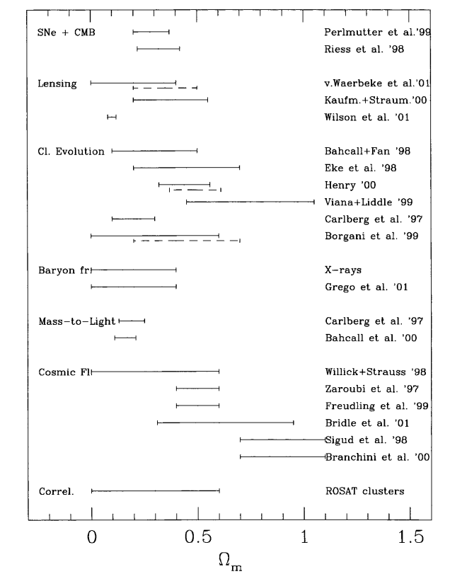
Figure taken from
Schindler, SSRv 100, 299 (2002)
... and not much has changed in the twenty-odd years since then, as these excerpts from a review article in 2024 reveal.
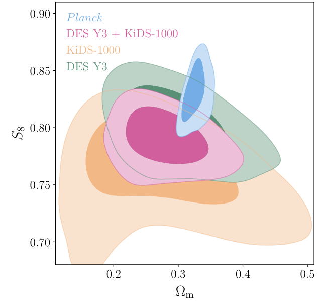
Figure 25.2 taken from
Lahav and Riddle, arXiv 2403.15526, 2024
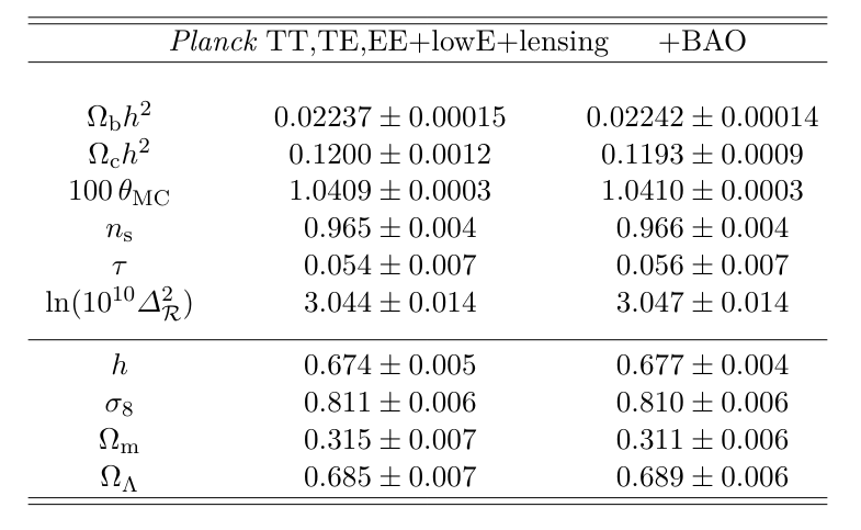
Table 25.1 taken from
Lahav and Riddle, arXiv 2403.15526, 2024
The conclusion is pretty clear: the average density of the universe is smaller than the critical density. That means that if the universe is as simple as we've assumed, it will expand forever.
Copyright © Michael Richmond.
This work is licensed under a Creative Commons License.