 Copyright © Michael Richmond.
This work is licensed under a Creative Commons License.
Copyright © Michael Richmond.
This work is licensed under a Creative Commons License.
Both stars and clouds of gas orbit around the center of the Milky Way; if we can figure out the properties of those orbits, we can learn something about the gravitational field of our Galaxy. However, due to their different sizes and shapes and electromagnetic signatures, astronomers need to handle the measurements of stars and gas very differently.
For relatively nearby stars, close enough that Gaia can measure parallax and proper motions, and for which we can determine radial velocity from Gaia or another telescope, we can figure out the full six-dimensional information:
Gaia (and associated followup surveys) has provided this data for tens of millions of stars. The exact results depend slightly on how one analyzes the dataset, but different groups have all reached roughly the same conclusion.
One way to characterize our Galaxy is by its rotation curve. Although some stars zoom in and out, from the inner regions to the outermost areas of the Milky Way, most move in orbits which are approximately circular and in the same direction. Plotting the speed of objects as a function of their distance from the center of the Galaxy yields the graph we call the rotation curve.
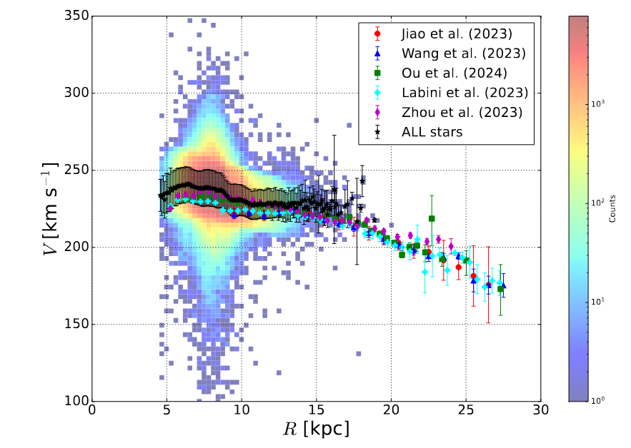
Fig 1 taken from
William, B., Mariateresa, C., and Gilberto, L. M.,
Journal of Cosmology and Astroparticle Physics,
Dec 2024
  The colored background in the graph above shows how many
     stars have been measured in each bin of radial distance
     and velocity.


  Q:  Why is there a region where the number of stars is very large?


  Q:  Why do the numbers decrease sharply for distances around 2-3 kpc
         from the center of that region?
The answer is that our Sun is located at the center of the region, about 8 kpc from the center of our Galaxy. The main instrument used to collect this data, Gaia, becomes significantly less precise at distances beyond 2 or 3 kpc. If we rely on Gaia to determine the properties to stars, we can only measure the rotation curve in the region
5 kpc ≲ R ≲ 11 kpc
If we wish to measure the rotation curve outside this small range, we need to find another way to estimate the distances or motions of stars.
The authors of Exploring Milky Way rotation curves with Gaia DR3: a comparison between ΛCDM, MOND, and General Relativistic approaches choose three different types of tracers to help them extend their study of the rotation curve.
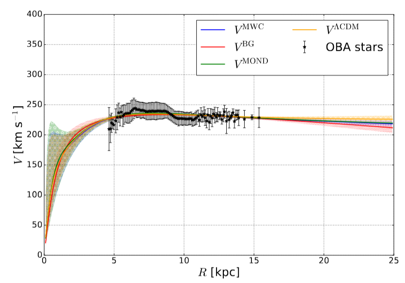
Fig 3a taken from
William, B., Mariateresa, C., and Gilberto, L. M.,
Journal of Cosmology and Astroparticle Physics,
Dec 2024
The good news is that Cepheids are luminous enough to provide information to large distances -- this version of the rotation curve reaches out to nearly 20 kpc from the center of the Milky Way. The bad news is that the number of Cepheids is relatively small, which leads to wider bins in distance and larger uncertainties in each bin (this study includes only 1705 Cepheids, vs. 242,000 OBA star).
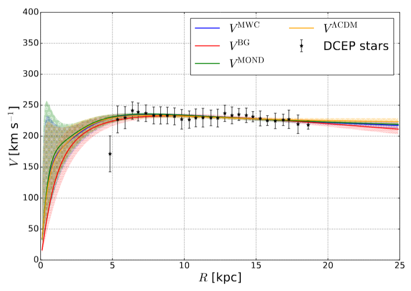
Fig 3b taken from
William, B., Mariateresa, C., and Gilberto, L. M.,
Journal of Cosmology and Astroparticle Physics,
Dec 2024
The most massive and most luminous of the red giant stars evolve relatively quickly from massive main-sequence stars. If one can isolate these young RGB stars from the (many, many) olders ones, then one can again assume confidently that they move in circular orbits near the plane of the Milky Way. Since there are a lot of these stars (475,000 in this study), the statistical uncertainties in the results are small.
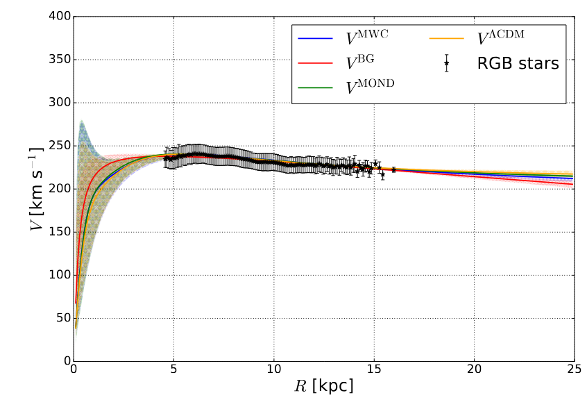
Fig 3c taken from
William, B., Mariateresa, C., and Gilberto, L. M.,
Journal of Cosmology and Astroparticle Physics,
Dec 2024
No matter which tracer we choose, the shape of the extended rotation curve of the Milky Way seems clear: nearly flat, but with a slight decrease in speed at larger galactocentric distances. The fact that all three tracers agree with each other is a good sign that our conclusions are firm.
But we can't become too confident: there are several different types of error that can creep into our calculations. A paper by Eilers et al. (2019) describes in detail how various factors can affect the results (see Section 5.2 in particular). Many of the calculations depend upon the density distribution of the stars being used as tracers -- we need to correct the observations for incompleteness and bias to interpret them properly. Although the uncertainty in the rotation speed is just a few percent in the solar neighborhood, it increases rapidly as one looks farther and farther away.
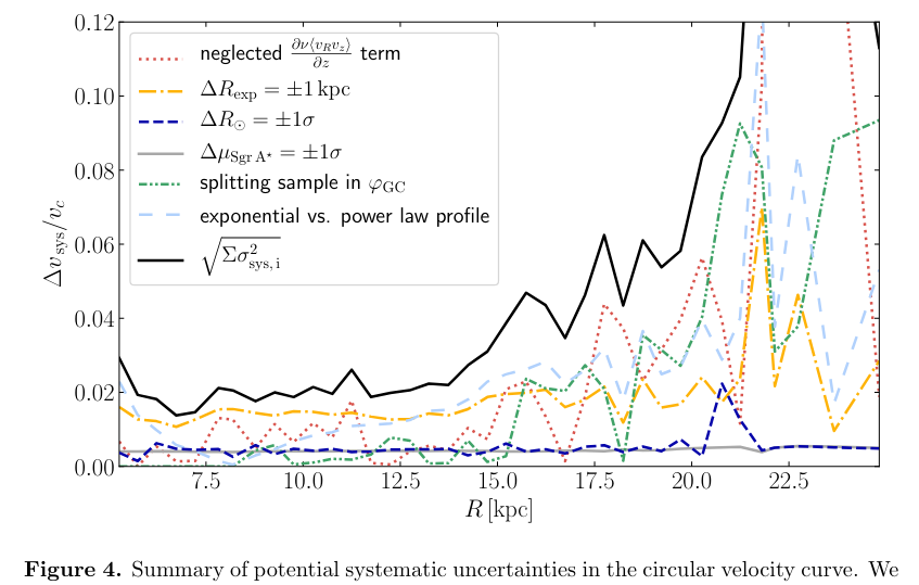
Fig 4 taken from
Eilers, A.-C., et al., ApJ 871, 120 (2019)
So, we've done the best we can using stars to map the motions of objects in the Milky Way's gravitational field. Even using a number of special stars -- Cepheids or young red giants -- we are still somewhat limited because Gaia can measure accurate parallaxes only for stars within a few kpc of the Sun's location; morever, clouds of gas and dust block our views of the inner Galaxy.
Is there a better way?
Instead of measuring stars,
could we look at gas in the Milky Way?
We'd have to apply very different techniques:
gas exists in very large, diffuse clouds,
most of which emit little or no optical light.
It's just not possible (*) to measure the parallax to these clouds
in the same way that we measure the parallax to stars.
(*) Well, there are a few exceptions for masers
On the bright side, the 21-cm emission from clouds of neutral hydrogen does provide a few nice features to astronomers:
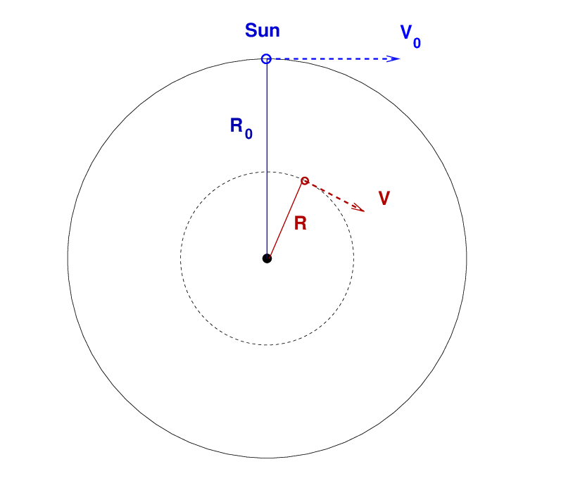
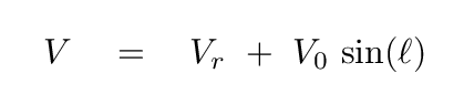
Let's consider measuring the radial velocity of clouds of gas which are located closer to the center of the Milky Way that the Sun. The diagram below shows a bird's-eye view of the Galaxy, looking down from above the galactic North Pole. The Sun orbits at a distance R0 at a speed V0, while one particular cloud of gas orbits at a distance R with a speed V.
Now, suppose we point our radio telescope at the cloud, which is located at galactic longitude ℓ. When we tune out telescope to the 21-cm emission line of neutral hydrogen, we won't measure the orbital speed V directly. Instead, the wavelength of the emission from this cloud will be shifted by the radial velocity Vr, which is simply the difference of the radial components of V and V0 along the line of sight.
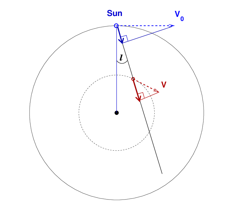
Figuring out the sizes of these radial components of each velocity is rather involved; see your textbook or, for example, Peter Kalberla's guide to the analysis of 21-cm line profiles. Today in class, we'll consider just one particularly simple case: a cloud which is moving directly away from the Sun along the line of sight. As the diagram below shows, the orbit of this cloud must be tangent to the line of sight of our radio telescope.
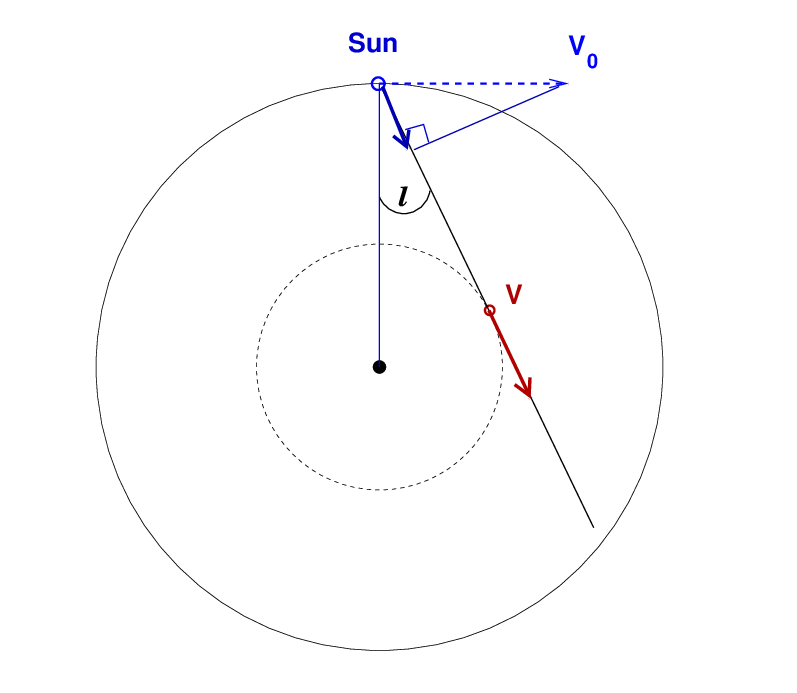
For this situation, the cloud will have the largest radial velocity of any clouds along that line of sight (if we ignore clouds of gas which are on the "far side" of the Galaxy, outside the Sun's orbital radius). That's handy: our telescope may detect a number of clouds, all at different locations, moving in different orbits, but the cloud with the largest velocity will (almost) always be the one in an orbit tangent to the line of sight.
Moreover, the orbital speed of this cloud is relatively simple to compute:
We can even figure out the orbital radius, R, of such a cloud pretty easily.
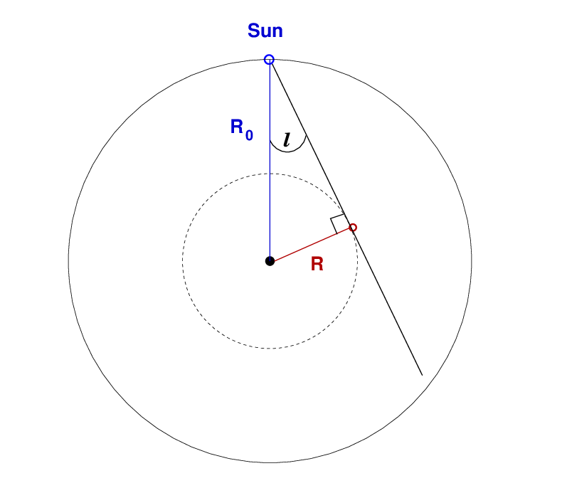
   Q:  Can you write an expression for the distance of the cloud
          R in terms of other quantities?
All the diagrams and equations above leave the properties of the Sun's orbit as symbols. In order to perform calculations, one must adopt some values. As described in Sofue (2017), astronomers have decided to adopt "official" values for these quantities to simplify the comparison of results by different groups. The "official" values may not be exactly correct, but they are close to the actual ones and easy to remember. For reference, the "traditional" values are
Recent measurements suggest that the true rotational velocity is a bit higher, perhaps around 235 km/s, but that's no big deal.
Let's try to put all this information about the motion of gas into practice. The EU-HOU collaboration has created a website which allows students to "measure" the 21-cm emission line at any location in the Milky Way, and has written materials to explain how one can use these measurements to make a rotation curve.
Visit the URL above and click on the "HI profiles" link. You should see a new webpage which includes a box like this:
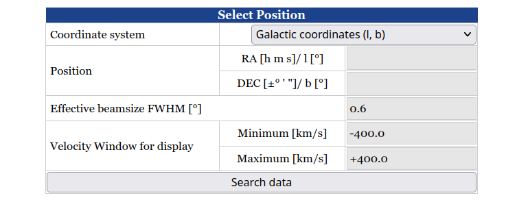
Enter a galactic longitude and latitude into this box, then click on "Search data". After a brief wait, you will be shown actual measurements of the radio emission in that direction from the Leiden/Argentine/Bonn (LAB) Survey of Galactic HI, based on observations made with a pair of big (diameters of 25 and 30 meters) radio telescopes in the years between 1989 and 2000.
In addition to a graph showing the intensity as a function of radial velocity,
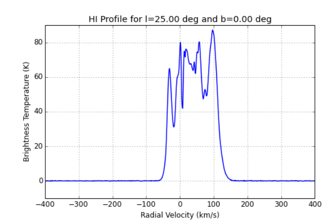
you can download an ASCII text file with the values in order to make your own graph.
![]()
In most cases, clouds which are on the orbit tangent to the line of sight will have the largest positive velocity in each profile.
If we split up into groups and share the work, perhaps we can make our own rotation curve of the inner Milky Way, and compare it to those in the literature.
galactic longitude   orbital radius     radial velocity     orbital velocity
      ell                  R                  V_r                V(R)
    (degrees)            (kpc)              (km/s)              (km/s)
-----------------------------------------------------------------------------

       15

       20

       25

       30

       40

       50

       60

-----------------------------------------------------------------------------
How does this rotation curve compare with the examples shown earlier in this lecture?
Copyright © Michael Richmond.
This work is licensed under a Creative Commons License.