Copyright © Michael Richmond.
This work is licensed under a Creative Commons License.
Copyright © Michael Richmond.
This work is licensed under a Creative Commons License.
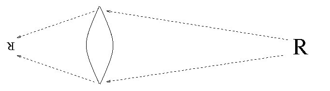
What is a lens? It's a piece of glass or other transparent material shaped so that light rays which pass through it are "bent", or diverted from their original paths:
Light rays "bend" when they pass through a transparent material because they travel a bit slower inside the material. Is there any other way to "bend" light rays?
Yes! Gravity can alter the path of light rays, too. A black hole, after all, is simply an object with a gravitational field so strong that even photons are unable to escape from its vicinity. Any light ray which attempts to fly outwards from a black hole is stopped, and turned back into the black hole. That's an extreme case of "bending."
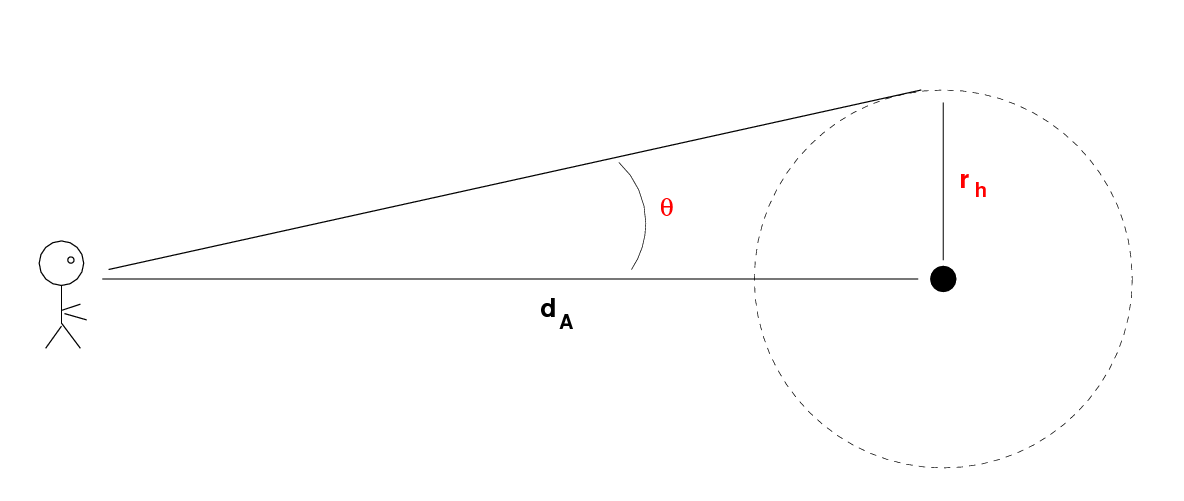
But there are more modest situations, in which the photon isn't stopped dead, but merely nudged a bit so that its direction (and energy) change slightly. For example, if we place a very massive object near the path of an incoming light ray:
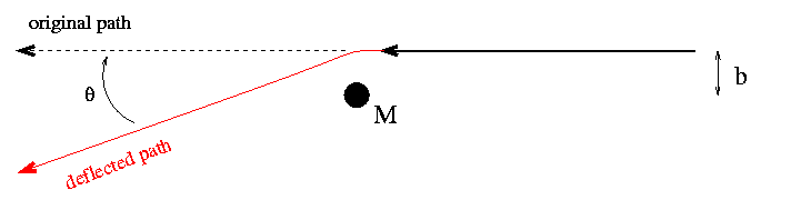
The angle theta by which the light ray is deflected depends on two factors: its closest approach to the massive object (called the impact parameter, and denoted by b in the diagram), and the mass of the lensing object, M. As you might guess, it takes both a very massive lens, and a very close approach, to cause any significant deflection.
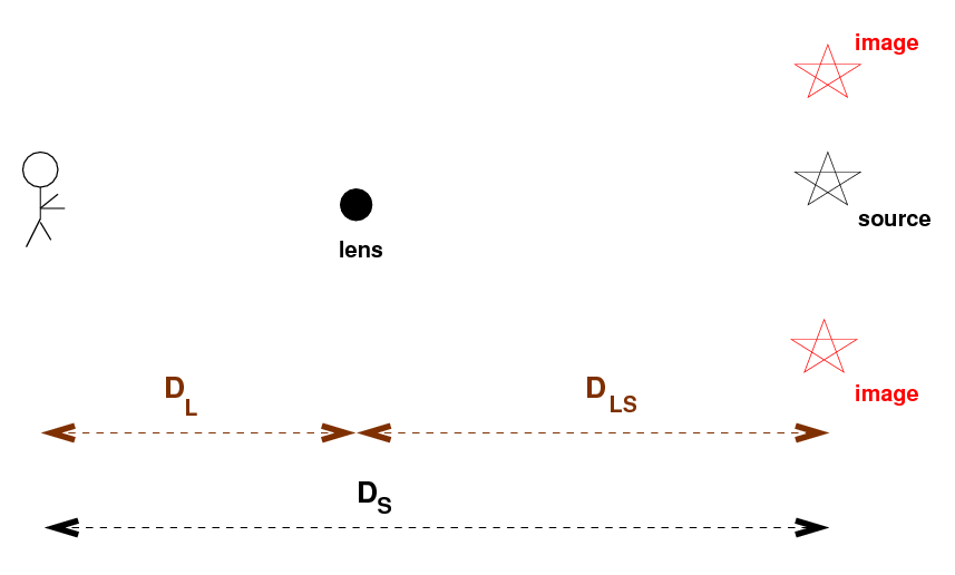
If an intervening mass lines up perfectly with a background source, it can bend the light from the source which would otherwise go far above us to come to us; and bend the light which would otherwise go far below us to come to us.
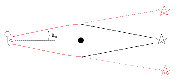
To us, it looks like there is light coming from an angle theta E above the actual source ... and from an angle theta E below the actual source ... and, in fact, from an angle theta E to the left, and the to the right, and everywhere in between. The result is that we see a ring of light surrounding the actual position of the source:
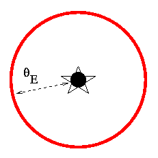
The angle theta E is called the Einstein ring radius, because Albert Einstein was the first to figure out that -- in the very unlikely event that a faint, massive object lined up exactly in front of a bright, background source -- we might see a bright ring of deflected light.
The Einstein ring radius depends on the mass of the lensing object: the more massive it is, the larger the Einstein ring radius. It also depends on the distance between us, the lensing object, and the background source. Gravitational lensing is most effective (meaning the ring radius is largest) when the lensing object is half way between us the and background source. In that event, the Einstein ring radius is given by this equation:

where
    G    =     gravitational constant
         =     6.67 x 10^(-11)  N*kg^2/m^2

    M    =     mass of lensing object, in kg

    D    =     distance from us to lens (and lens to source), in m

    c    =     speed of light
         =     3 x 10^8 m/s
This turns out to be pretty darn small.
mass of lensing object    distance         Einstein ring radius
 (solar masses)          (parsecs)       degrees      arcseconds
--------------------------------------------------------------------
lensed by a star
       1                    100         0.0000025      0.0089
                          1,000         0.00000078     0.0028
                         10,000         0.00000025     0.00089

lensed by a galaxy
    1 x 10^12           100 Mpc         0.0025         8.9
                      1,000 Mpc         0.00078        2.9
                     10,000 Mpc         0.00025        0.89

lensed by a galaxy cluster
    1 x 10^15         1,000 Mpc         0.025         89
                     10,000 Mpc         0.0078        28
                    100,000 Mpc         0.0025         8.9
Now, in general, the lensing object does NOT lie exactly half-way between the source and the observer, so the geometry is more complicated: there are three distances we need to consider, not just one.
If we can
then we can make a good model of the system. One of the (many) problems in this approach is determining the absolute mass of the lensing object(s). In some cases, the best models can be fit with a range of masses, corresponding to a range of distances.
Is there some way to break the degeneracy? In other words, is there some way to establish unambiguously the mass of the lensing object and distance to the lens and source? The answer is yes, if we can detect variations in the relative brightness of the images.
For example, consider the system RXJ 1131-1231. A long exposure with HST shows a bright, compact source with some fainter stuff around it:
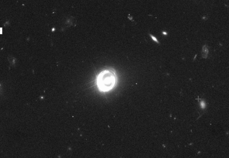
Image generated by the
Hubble Legacy Archive
But if we modify the contrast and zoom in on the object, we find a galaxy surrounded by a ring of light
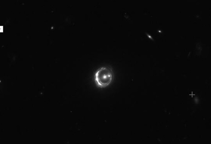
Image generated by the
Hubble Legacy Archive
and that ring has four point sources:
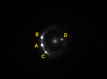
Image generated by the
Hubble Legacy Archive
In this instance, the central, diffuse object is a galaxy at a redshift z = 0.295 acting as a lens; and the four point sources are images of a background quasar at z = 0.658.
If one measures the brightness of each of the four images of the quasar over a long period, one will see gradual changes: the quasar itself has a luminosity which varies, as many do. But the four different images don't all appear to change at exactly the same time:
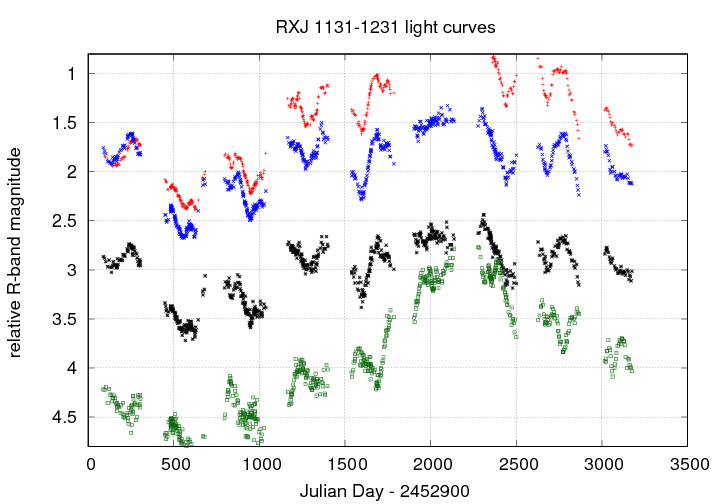
Data taken from
Vizier and Tewes et al., A&A 556, A22 (2013)
  Q:  Can you figure out the time delay between the image
      shown in green and the other images?

      Grab the data from the link below.  The Julian Date is in column 1,
      and magnitudes for images A, B, C, D are in columns 2, 4, 6, 8,
      respectively.

           data file for RXJ 1131-1231 from Tewes et al. (2013)
My quick attempts yielded a delay of about 90 days between the variations in the three brightest images (A, B, C) and the faintest image (D). Suyu et al., ApJ 766, 70 (2013) find a delay of 91.4 +/- 1.5 days.
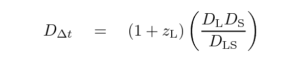
If one can measure a time delay between images, and one has a good model for the mass of the lensing object(s), and one has the redshifts of the lens(es) and the source, then one can figure out the distance to each object; or, if one wishes, one can set constraints on various cosmological parameters. Suyu et al., ApJ 766, 70 (2013), for example, create a model with 39 (yes, 39!) parameters and perform many complex calculations to place constraints on them all. Their estimate for the "time-delay" distance for this object
is roughly 2100 Mpc.
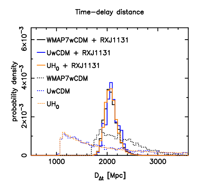
Taken from Figure 7 of
Suyu et al., ApJ 766, 70 (2013)
Moreover, they believe that this measurement of a really, really large distance has a small uncertainty:
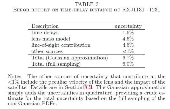
Table 3 taken from
Suyu et al., ApJ 766, 70 (2013)
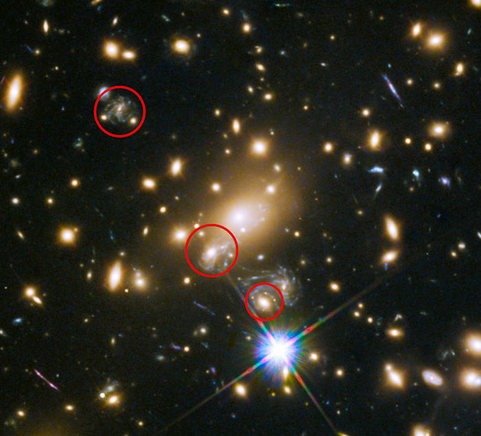
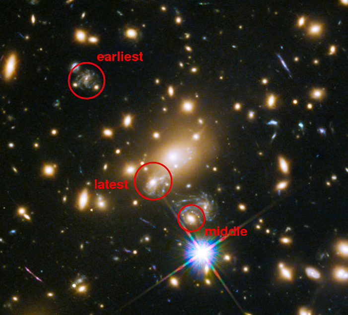
In 2014, astronomers noticed a fortunate but improbable event, behind a mass clusters of galaxies called MACS J1149.5+2223 were a number of background galaxies. Some of these galaxies were lensed, creating multiple images.
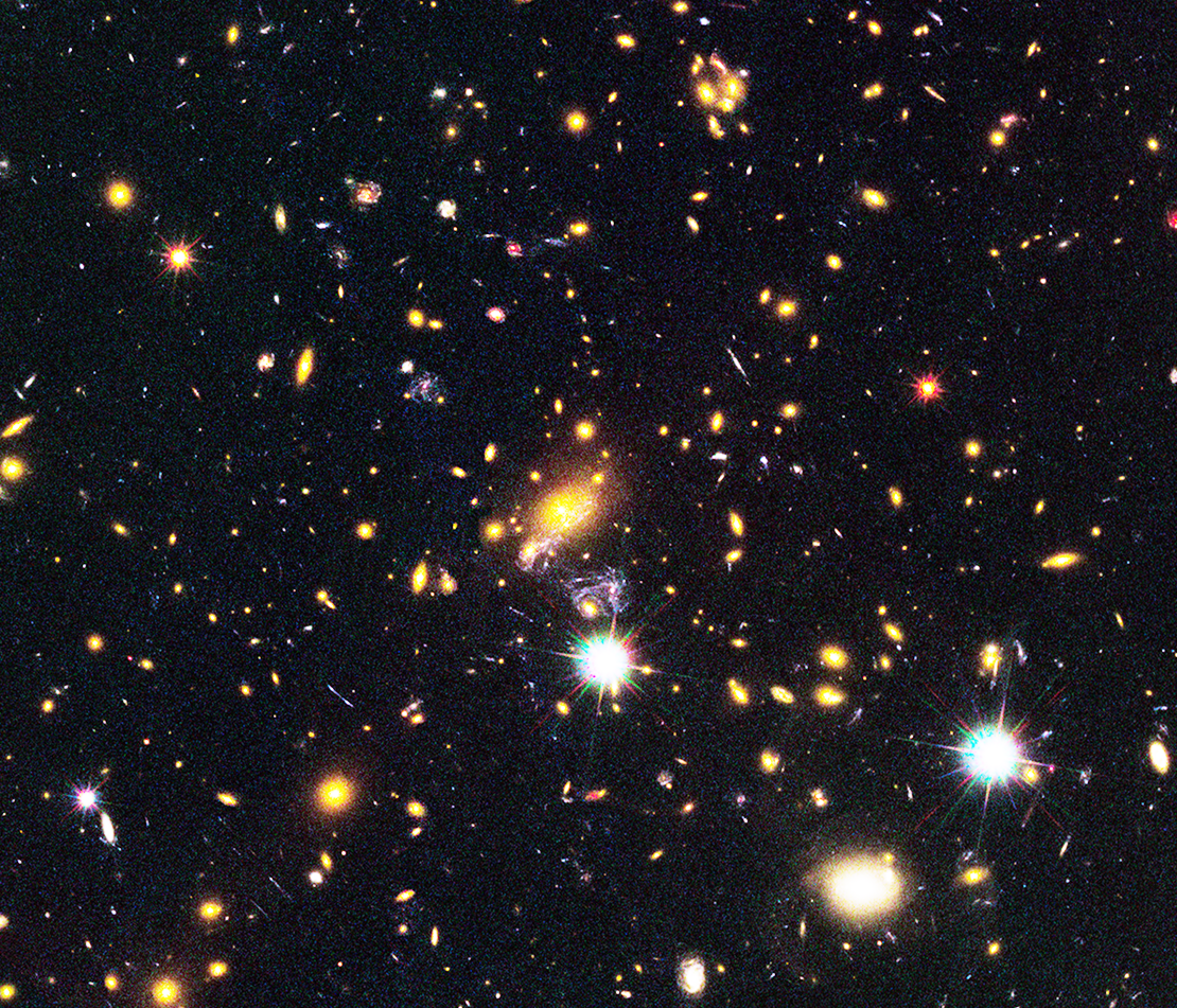
Image courtesy of
NASA, ESA, and M. Postman (STScI), and the CLASH team.
Let's zoom into the central region.
Q: Can you find three images of the same blueish galaxy?
There are many, many galaxies in this cluster, so making a model of the gravitational lensing is ... complicated. Nonetheless, some astronomers tried to account for the effects of all the galaxies, as well as the diffuse mass of the hot gas spread throughout the cluster. Grillo et al., ApJ 822, 78 (2016) identify all these objects (and more) as members of the cluster and place them into their model -- which ends up with 300 cluster galaxies and 3 concentrations of dark matter.
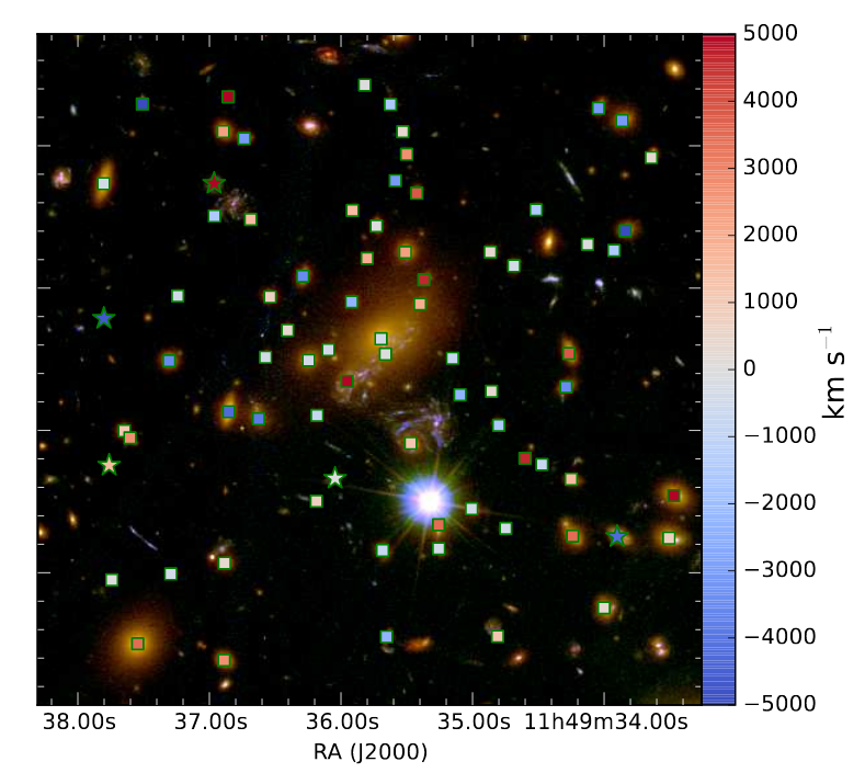
Taken from Figure 2 of
Grillo et al., ApJ 822, 78 (2016)
One can follow the light paths from the background galaxy through this model -- which includes distances to the lensing objects and background source objects -- and predict the time it takes light to travel along each path. The results are a bit counterintuitive: the closer the path is to the center of the system, the LONGER it takes light to travel.
Now, in 2014, something happened in this region of the sky: a supernova appeared, exploding within the highlighted background galaxy. Astronomers grew excited, because they realized how important a gravitationally lensed supernova could be. Back in 1964, Sjur Refsdal had described how a gravitationally lensed supernova might be used to measure very large distances. To honor his idea, this supernova became known as "SN Refsdal".
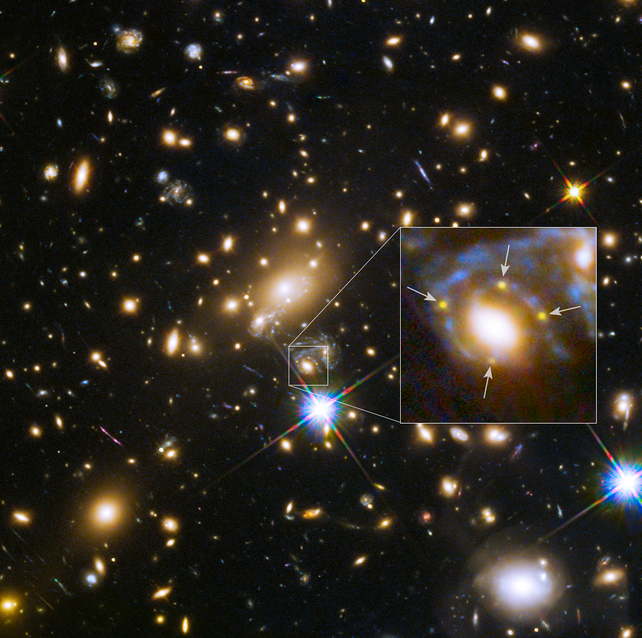
But we did not see just one image of this supernova -- we detected FOUR!
Look closely at the southernmost image of the lensed galaxy, in an image taken in November, 2014 (click on it for a larger version). One of the spiral arms of a distant, blueish, background galaxy happens to sit directly behind a reddish elliptical galaxy in the cluster ... and in that spiral arm, a supernova exploded!
Three of the SN images are easy to see, but the fourth one is a bit fainter. It helps to subtract away a model of the cluster galaxy which lies right in front of the background galaxy's spiral arm containing the SN.
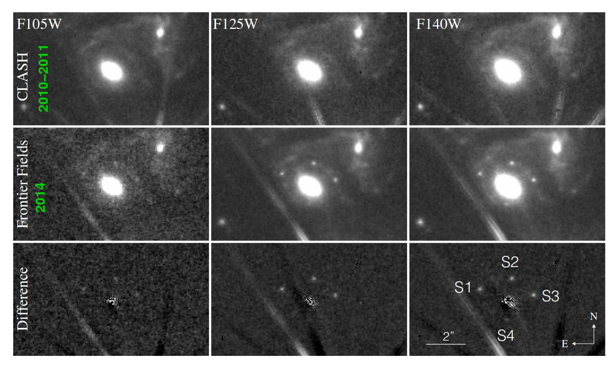
Image taken from Fig 1 of
Kelly et al., Science 347, 1123 (2015)
Because HST took several images of this region during 2014, scientists were able to determine
Putting this information into their models, Kelly et al., Science 347, 1123 (2015) examined the light-travel times along the paths to the other two locations of this galaxy. They suggested that light from the supernova might appear in the "middle" copy of the spiral galaxy at a future time, within a year to a decade from now (2015 to 2025).
Grillo et al., ApJ 822, 78 (2016) studied this system more carefully (with more time), and made (among other claims) one post-diction and one pre-diction. First, the light from this supernova should have appeared in the northernmost image of the galaxy about 6000 days ago, around 1995; but we don't have any images of this region taken at that time with sufficient detail to confirm this claim.
Second -- and more exciting -- they made a rather precise PRE-diction: according to their model, light from the SN would appear in the middle image of the galaxy at some point in the not-too-distant future: Their first attempt made a prediction that the delay would be "about a decade", but their second version (see Table 5) shows the delay between image S1 and the central location to be between 328 and 390 days.
  Q:  If the image S1 was first noticed in November, 2014,
      when should an image of the SN appear in the middle location?
Grillo et al. submitted their paper to ApJ on 2015 November 12 (and it was received on 2015 November 15), so ... barely in time to make a real prediction. But they did.
So, what happened?
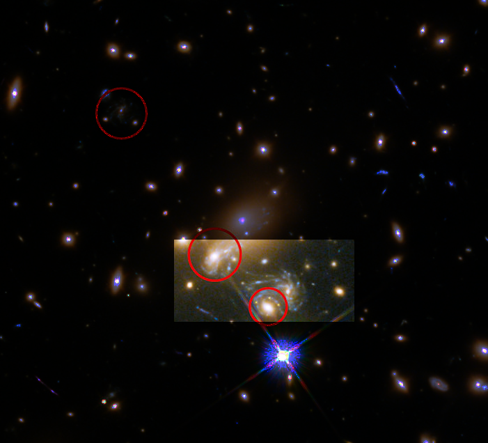
Let's zoom into this little region within the cluster, containing the two images in question.
The image below (click to animate) will show this region of sky in pictures taken in 2011 (before the four images), in Apr, 2015 (soon after the four images appeared), and then again in Dec, 2015.
Image taken from 1 of
Kelly et al., ApJ 819, 8 (2016)
In December, 2015, the four SN images in the southernmost copy of the galaxy were fading -- but a new image (called "SX" in the pictures above) appeared in the central copy of the galaxy -- just as predicted, in time as well as in position:
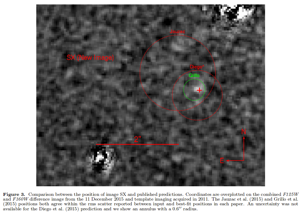
Figure 3 taken from
Kelly et al., ApJ 819, 8 (2016)
Hooray!
Light curves of the four images around the southern copy suggest that this was a Type IIP supernova, not very luminous, perhaps a distant cousin of SN 1987A.
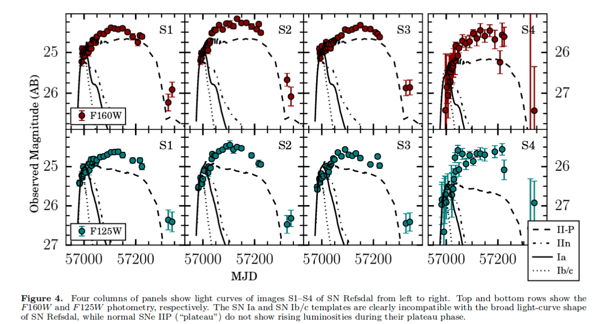
Figure 4 taken from
Kelly et al., ApJ 831, 205 (2016)
Chances are slim that we will catch many gravitationally lensed supernovae exploding over the next few decades, but since we can in theory detect them far beyond redshift z=1, they provide a mean to measure distances more deeply into space than any other method in our toolbox.
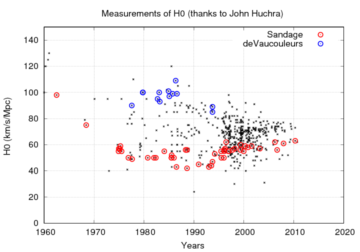
Astronomers have been measuring the value of the Hubble Constant H0 for many years -- and disagreeing with each other about its value for just as long. John Huchra collected many published measurements over the years, and I've plotted some of them below:
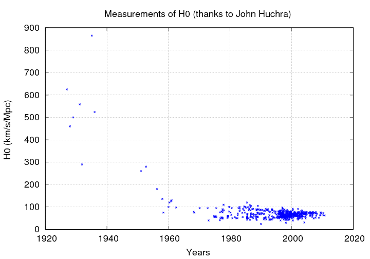
Note the general trend to smaller values, reaching a relatively steady "valley" around 1960. But for the next few decades, there was a rough split in the community between the "long" and "short" camps.
The split was in part due to different methods, but also in part due to a clash of certain individuals.
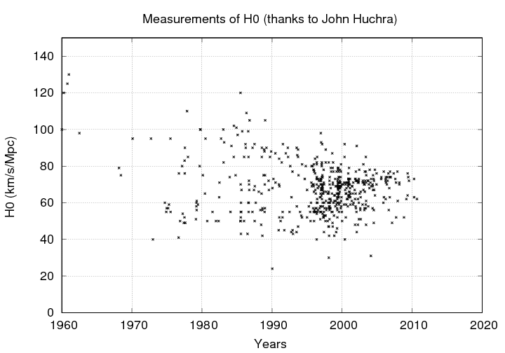
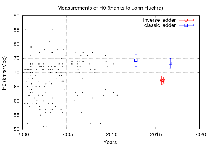
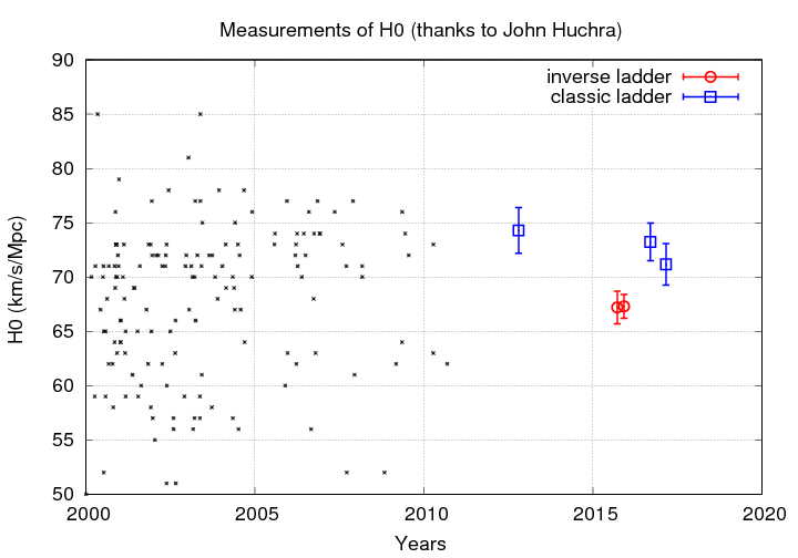
In the past decade, estimates have started to converge around 70 ... but there is now a new, much smaller split which is driven by the starting point of the technique:
Note that each method yields results with very small uncertainties (that's good), but the results don't agree within those uncertainties (that's bad).
Earlier this year, Jang and Lee, ApJ 836, 74 (2017) used a somewhat slim version of the classic ladder, employing TRGB to determine the distances to 6 galaxies which hosted good, low-reddening examples of Type Ia SNe. They derived a value which may start to close this gap.
But just how does the "inverse ladder" technique work? Is it better than the "classic ladder" which we have discussed? Should we expect it to give us the same result?
Let me try to explain the basic idea behind this completely different method for measuring distances. I'm no expert at it, so I may make some mistakes.
Way back in the very early universe, when it was still so hot that all the matter was ionized, there was a mix of dark matter, baryonic matter, and photons (and neutrinos, but we'll ignore them for now). Overall, the density of this mixture was relatively uniform; but there were some places which were a little more dense than usual, and some which were a bit less dense.
The overdense regions generated regions of higher pressure. The dark matter simply settled into the center of each dense region, because it interacted with the rest of the mixture only via gravity; but because the baryonic matter (gas) and photons could push and pull each other via electric forces, they reacted to pressure by expanding outward. So, around each overdensity, a wave of (gas + photons) spread out at high speed, roughly half the speed of light. Because the gas was ionized, it was opaque, and trapped the photons; the gas "went along for a ride" as the photons spread outward.
Animation courtesy of
Ned Wright's Cosmology Pages
When the temperature of the universe dropped to about 5000 degrees or so, the electrons and protons combined to form neutral hydrogen -- which is transparent to most radiation. Suddenly, the photons could pass through the gas and fly off on their own.
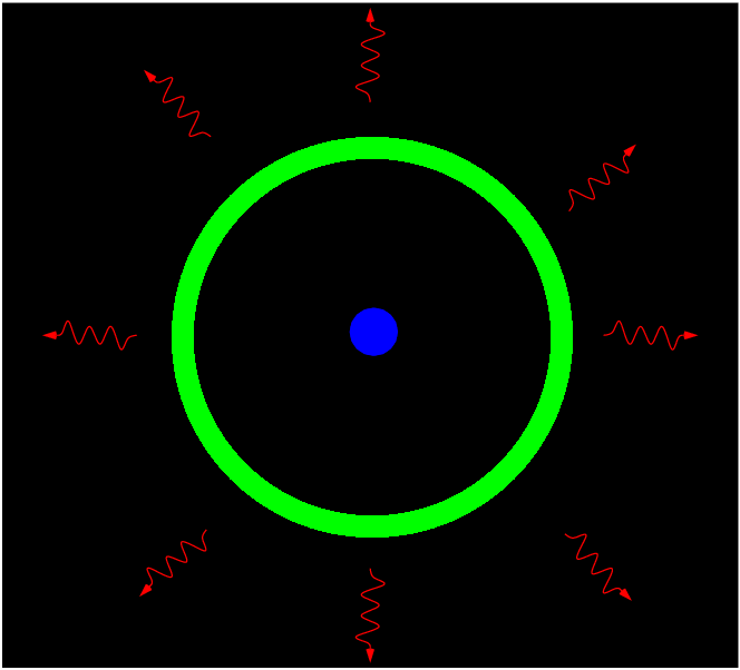
The baryonic matter was left sitting in a big shell around the dark-matter core of each overdense region.
The result: a very young universe in which there are a bunch of "nuggets" of dark matter, each surrounded by a shell of baryonic matter of a roughly similar size.

Image courtesy of
BOSS project
The escaping photons carry with them a ghostly picture of these shells -- and that's what we see when we examine the Cosmic Microwave Background closely.
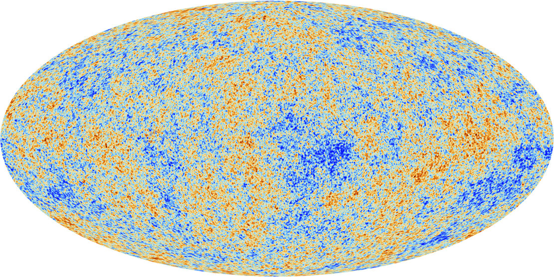
Image courtesy of
ESA and the Planck Collaboration

Image courtesy of
Galaxies and Cosmology 2015
One way to measure the size of these shells in the early universe is to compute the power spectrum of the fluctuations in the CMB. The big bump is the "first acoustic peak", which corresponds to angular size of the shells.
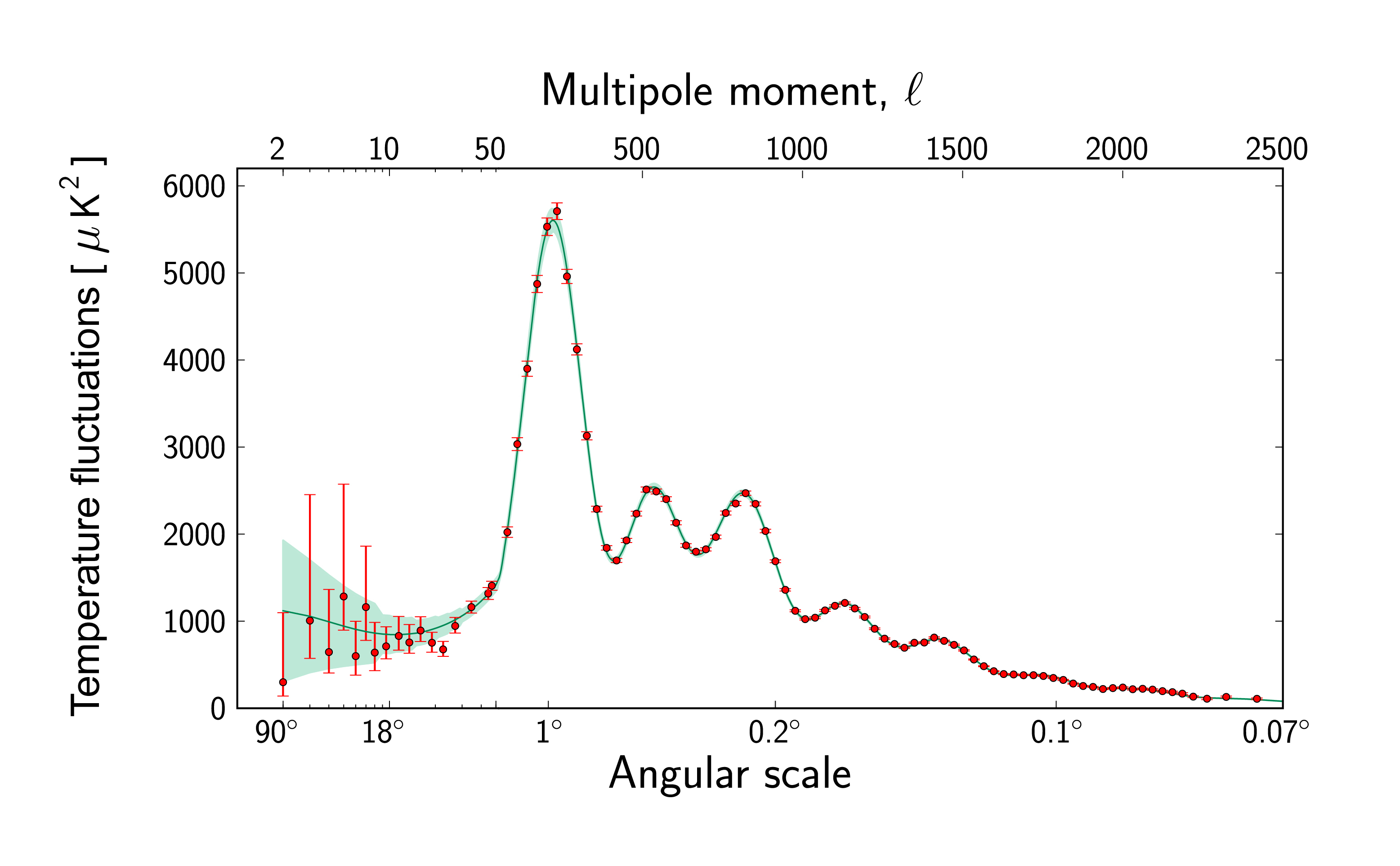
Image courtesy of
ESA and the Planck Collaboration
The remnants of these shells provide a "ruler", which can be identified in the modern-day universe by measuring the two-point correlation function of galaxies.

Image courtesy of
NASA’s Wilkinson Microwave Anisotropy Probe, Sloan Digital Sky Survey,
and Laurence Berkeley Laboratory
Evidence for these ghost-shells in the local galaxy population was first detected by the SDSS survey back in 2005.
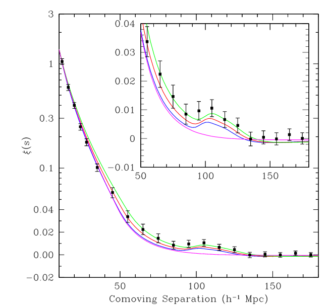
Figure 2 of
Eisenstein et al., ApJ 633, 560 (2005)
and confirmed by later surveys.
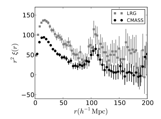
Figure 16 of
Anderson et al., MNRAS 427, 3435 (2012)
So, how does this help us to measure distances? Again, I'm not an expert in this technique, but I believe that it goes something like this:
Now, in practice, we need to include galaxies within a range of redshifts in order to create a sample large enough to show the bump in the 2-point correlation function due to the shells. The measurements of the angular sizes have some uncertainty as well, as do the other calculations mentioned in this procedure above. A recent paper shows the diagram below to indicate how one can fit models of the universe's expansion to the BAO data (shown as blue symbols) and SN data (black symbols) to determine the value of H0 at the current time. As you can see, the BAO measurements have pretty large uncertainties, due in part to the relatively small volume of space and small number of "shells" within that space; using SNe to measure RELATIVE distances as a function of redshift and fitting the SN data to the BAO data helps to pin down the extrapolation to z=0.

Figure 5 from
Aubourg et al., Phys Rev D, 92, 123516 (2015)
So, that's the basic idea. The inverse ladder starts at very high redshift -- where physics is simple (so I am told), and works it way back toward us here on Earth. The classic ladder starts on Earth itself, orbiting around the Sun, and works its way out, using stars (inside which physics is complicated) as markers. The two methods meet at redshifts around z=0.2 to 0.5, using type Ia SNe as the final step in each ladder.
But, alas, the two ladders don't yield the same result.
Now, there are a (at least) couple of possible explanations, some or all of which could be true.
If the entire universe is homogeneous, the properties of LOCAL and OBSERVABLE should be the same. But if there are small differences between one portion of the observable universe and another -- if, for example, one region is slightly more dense, and another is less dense -- then the expansion rates within those regions will be slightly different.
Copyright © Michael Richmond.
This work is licensed under a Creative Commons License.