 Copyright © Michael Richmond.
This work is licensed under a Creative Commons License.
Copyright © Michael Richmond.
This work is licensed under a Creative Commons License.
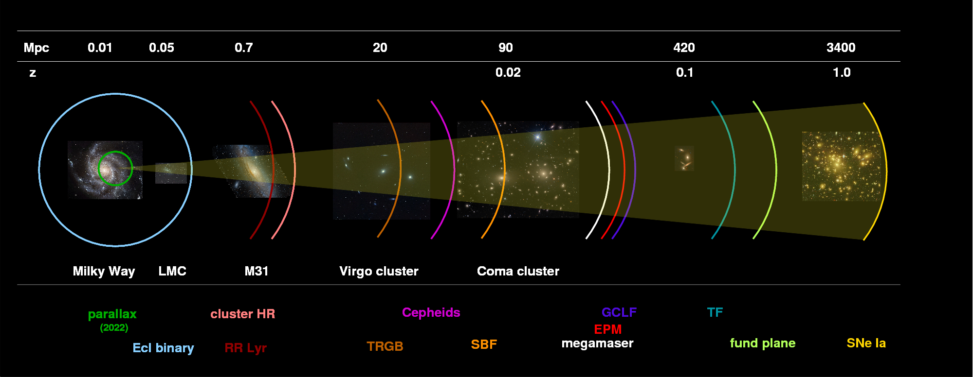
The methods we've described so far can only reach out to the nearest galaxy clusters. If we wish to probe deeper into the universe, we need to find new ways to estimate distances. The methods I'll describe today each have a strong point and a weakness.
The short answer is "a star which explodes."
Now, there are several mechanisms which cause a star to explode, and the pre-explosion object can have several different forms. We'll discuss some of those issues a bit later.
But from an observational point of view, a supernova is a star which suddenly appears in a galaxy, shines as brightly as an entire galaxy for a few weeks or months, and then gradually fades away. Here are a few nice examples of recent supernovae.
SN 2011 in M101
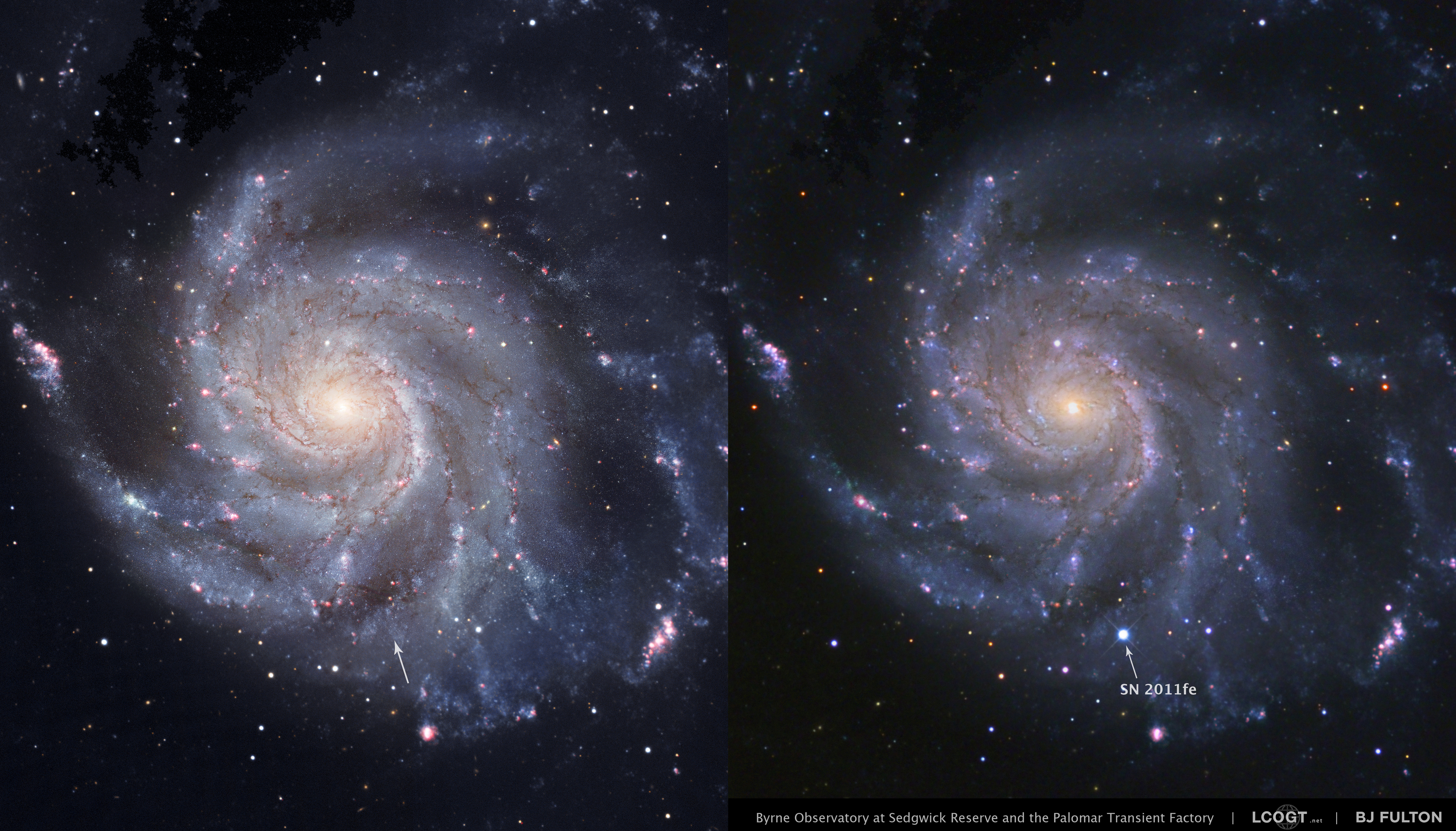
Images of SN 2011fe in M101 courtesy of
PTF and B. J. Fulton
SN 2014J in M82
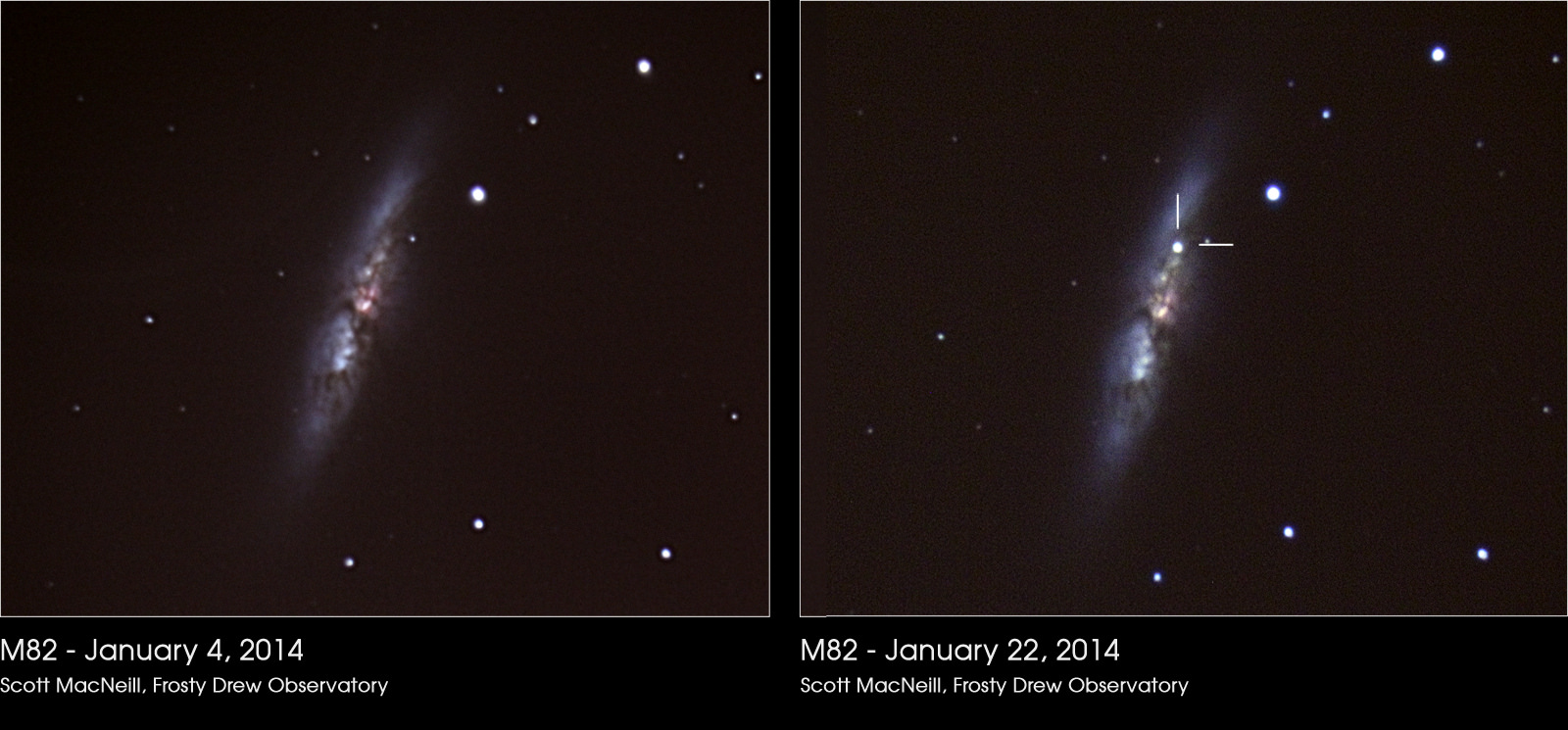
Images of SN 2014J in M82 courtesy of
Scott McNeil
SN 2017eaw in NGC 6946 -- which is bright right now!
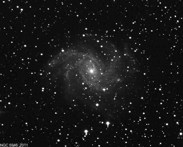
Image of SN 2017eaw in NGC 6946 courtesy of
Gianluca Masi and the Virtual Telescope Project
Now, these pictures don't really show how bright a supernova can be. In many cases, a supernova can outshine all the stars in its host galaxy for a brief period. For example, the earlier pictures of SN 2011fe in M101 give the impression that the SN was just one little blob of light among many others ...
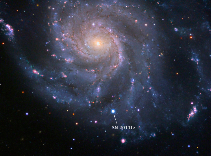
Image of SN 2011fe in M101 courtesy of
PTF and B. J. Fulton
and cropped by me.
But if one uses a little telescope, like my 12-inch Meade LX200 at the RIT Observatory, and takes only a short exposure, then we can compare the light from the galaxy's nucleus and spiral arms to that from the supernova more clearly. Below is an R-band (red light) image taken on Sep 25, 2011, when SN 2011fe was already past its peak brightness and starting to fade.
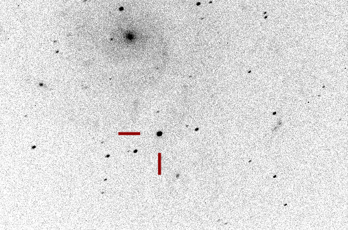
R-band image of SN 2011fe in M101 courtesy of
Michael Richmond and the RIT Observatory
And below is an image taken through a B-band (blue light) filter. The SN, all by itself, produces much, much more blue light than the billions of stars in the nucleus of this galaxy!
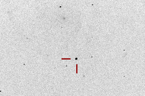
B-band image of SN 2011fe in M101 courtesy of
Michael Richmond and the RIT Observatory
This is even worse because SNe ...
The star "S Andromeda" was a type Ia explosion in the Andromeda Galaxy, but it happened just a few decades before astronomers were ready with equipment powerful enough to study it properly.
Thirty years ago, in 1987, a supernova appeared in the Large Magellanic Cloud. It was close enough that neutrinos from the explosion were detected on Earth, but no event since then has even come close.
There is a very wide variety of supernova classes and sub-classes. It's easy to get lost in the different types and designations. For our purposes, all those fine distinctions aren't necessary. Even though there APPEAR to be many different types, one can in the end separate them into just two varities.
Want some practice? Look at the following pictures, and try to separate the four different animals into two species. All the individuals pictured have two legs, one head, and stand about two meters tall.
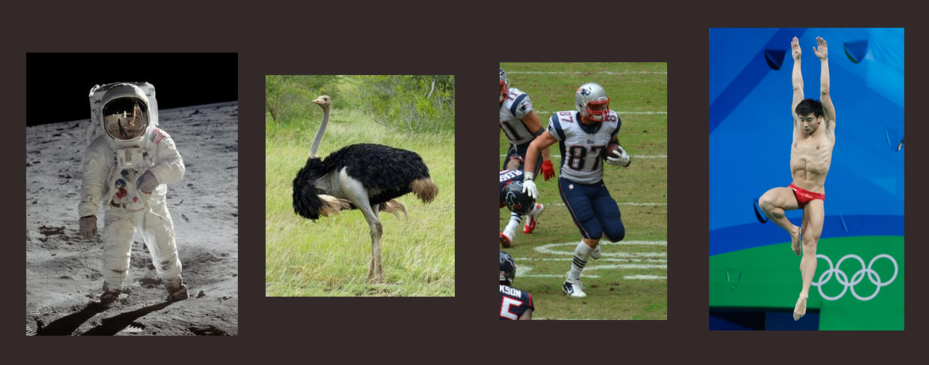
Image of ostrich courtesy of
berniedup and Wikipedia .
Image of Rob Gronkowski courtesy of
Wellslogan and Wikipedia.
Image of Apollo astronaut courtesy of
NASA.
Image of Cao Yuan courtesy of
Fernando Frazão/Agência Brasil and Wikipedia
(I hope you got this right)
There are just TWO species, even though all the pictures look quite different.
         Human                             Ostrich
  --------------------------------------------------------------
    hidden behind many layers of         covered by feathers
        spacesuit

    hidden under an NFL uniform
        and helmet

    not covered by clothing
  --------------------------------------------------------------
The three different humans LOOK different because they are wearing different amounts of material over their bodies; if you could slice each human in half, you'd find the same stuff inside: bone, muscle, blood, etc.
Well, it's the same thing with supernovae. There are just two varieties, really, but one of them wears quite a range of clothing.
        Massive Star Core                  White Dwarf
  --------------------------------------------------------------
     Type IIP  - hidden under thick            Type Ia
        envelope of hydrogen

     Type IIb  - hidden under a thin
        layer of hydrogen, covering
        thin envelope of helium

     Type Ib   - hidden under thin
        envelope of helium

     Type Ic   - hidden under a
        thin envelope of C, O, etc.
  --------------------------------------------------------------
and hundreds of other papers ...
but the end result is
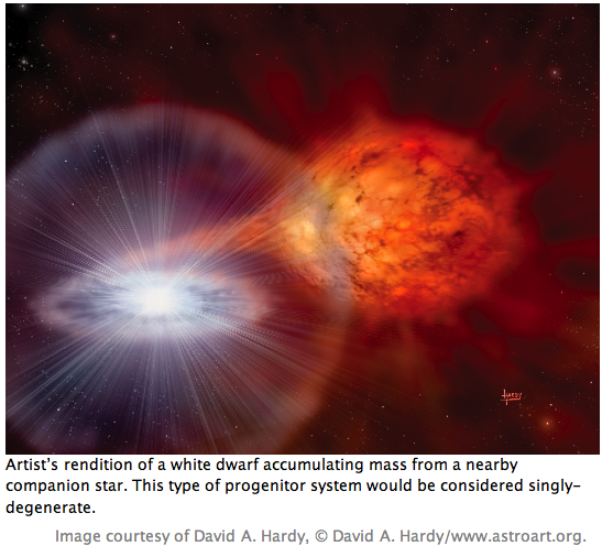
Well, that's one possibility. Another is that TWO white dwarfs in a close orbit may eventually merge (the double degenerate scenario). The merger creates a single object which again exceeds the Chandrasekhar limit, and, once again, Ka-Boom.
In this case,
In both cases, very roughly 1051 ergs of energy are released by the, um, complex processes occuring within the central regions of the progenitor star. So, to a very very rough approximation, in both cases, we see the same thing: an expanding cloud of extremely hot gas, flying outward at very high speeds, reaching absolute magnitudes of Mv ~ -17 to Mv ~ -21.
How can we use this big explosion to measure a distance?
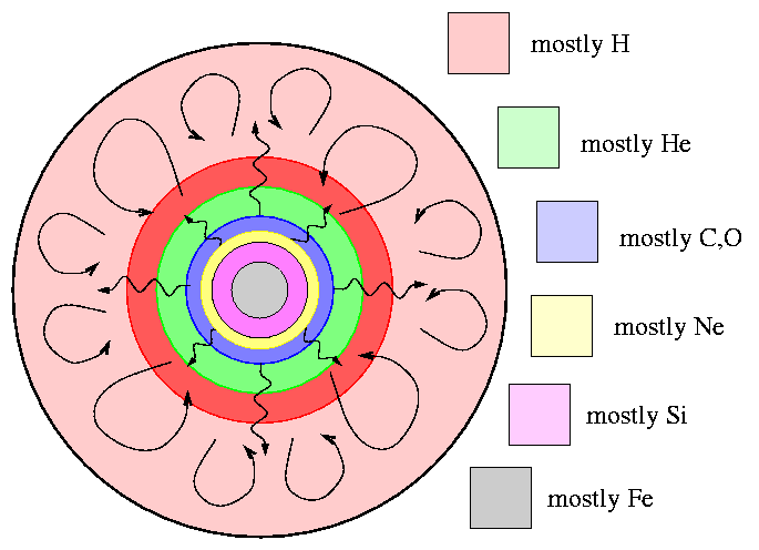
For measuring distances, we will concentrate on just one of the sub-types of the "Massive Star Core" supernovae. A Type IIP event involves the core collapse inside a star which still retains most of its massive envelope of hydrogen. In very simple terms, when the core collapses,
The shock wave heats the bulk of the star and accelerates it outward, to speeds far above the escape velocity. In a word, the star explodes. However, if one looks more closely, one finds that the velocities of different layers of the star vary in a systematic way: material from the inner regions has a relatively small velocity, while material from the outer regions has a relatively high velocity. We call this homologous expansion. (Click on figure below to animate)
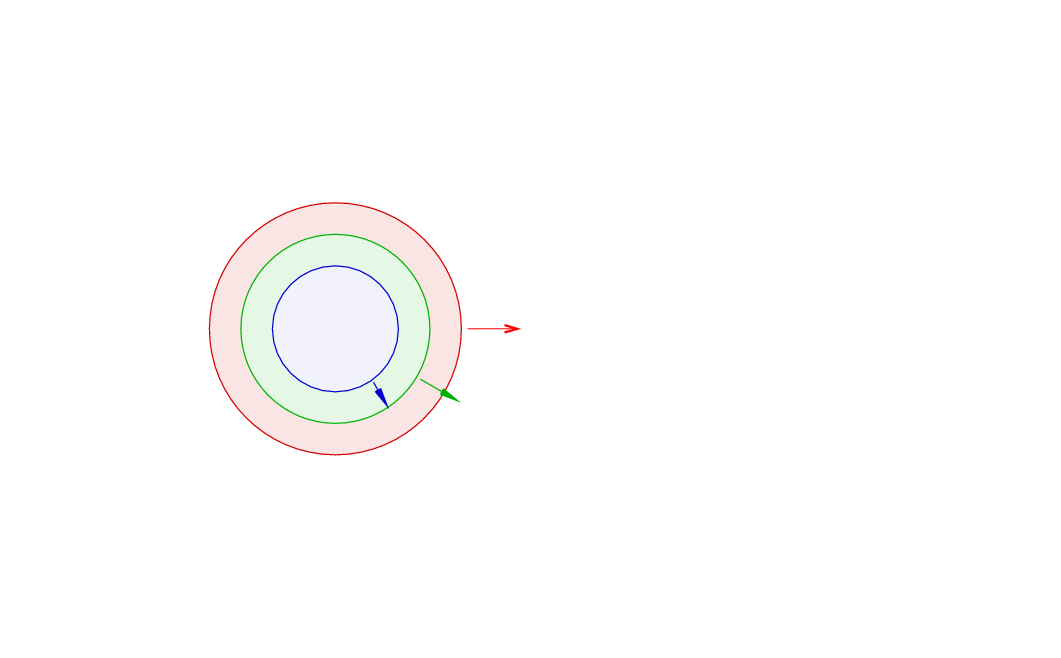
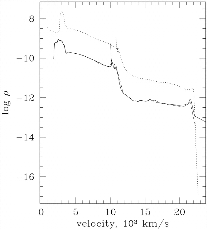
Figure taken from
Blinnikov et al., ApJ 496, 454 (1998)
The shock wave heats material up to very high temperatures, well over 100,000 Kelvin, ionizing all the hydrogen. The outermost layers emit X-rays and UV for several hours after the shock breaks out of the star, but then cool off quickly. When the temperature of the gas falls to roughly 6000 Kelvin, however, the hydrogen begins to recombine. At this point, as the outermost layer switches from ionized to neutral, its opacity drops: neutral hydrogen gas is MUCH more transparent than ionized gas.
When the outermost layer recombines, it becomes essentially transparent, and we can see into the layer below it. This layer is still hot enough that hydrogen is ionized ... but within a short time, it, too, cools off to about 6000 Kelvin and recombines. When it becomes transparent, we can then see into the NEXT layer of the star, and so on and so on.

The important facts here are
As time goes by, and we see further into the star, the velocity of this special layer will decrease. The graph below shows the evolution of a computer model of a Type II supernova -- the lines are drawn at roughly one-week intervals.
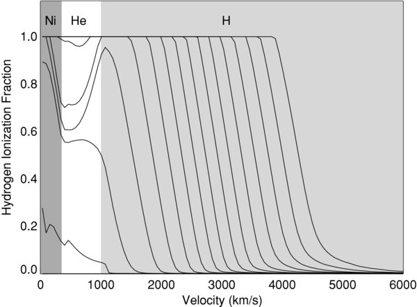
Figure taken from
Kasen and Woosley, ApJ 703, 2205 (2009)
The solid curve in the figure below shows the evolution of a computer model of an exploding star, while the circles show measurements of real supernovae.
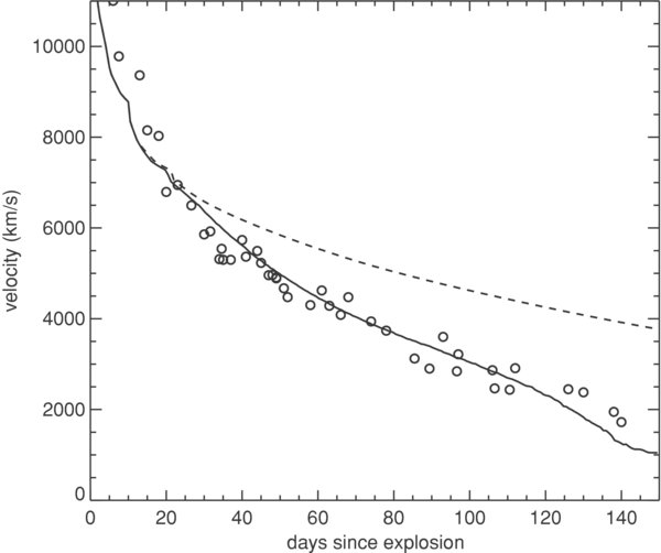
Figure taken from
Kasen and Woosley, ApJ 703, 2205 (2009)
The radius of any particular layer of material at some time t can be written as
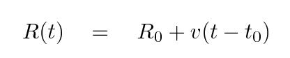
where t0 is the time of explosion and R0 is the radius of that layer at the time of explosion. With high-quality spectra of the supernova, we can measure the velocity of of one particular layer of the star -- the layer which happens to be acting as the photosphere at the moment.
Because the photosphere is in such a simple condition -- nearly pure hydrogen, at a temperature close to 6000 K -- it isn't too difficult to compute the radiation it emits. To first order, the photosphere acts like a "dilute blackbody", emitting flux
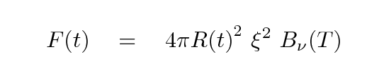
where T is the temperature ~ 6000 K, and ξ is a "dilution factor", inserted into the ordinary blackbody equation to account for several factors which cause the spectrum of the actual star to differ from that of a perfect blackbody.
Using spectroscopy and photometry, we can measure v(t) and the observed flux f(t). If we make measurements at several different times, when the photosphere has different sizes and luminosities, we have enough information to solve for the time of explosion, initial size of the star, and determine the distance as well; it's just a matter of comparing the luminosity F(t) to the observed flux f(t) and using the inverse square law (and hoping that there was no extinction, etc.).
It is a nice coincidence that the speed with which the recombination wave runs deeper into the star is very roughly the same as the rate at which the star is expanding; in other words, the radius of the apparent photosphere doesn't change a great deal while the wave is still moving through the envelope. As a result, the luminosity of Type IIP supernovae hits a plateau (hence the "P") and remains nearly constant for a month or two.
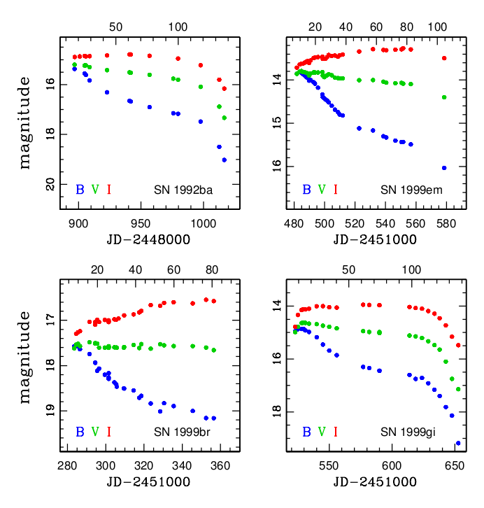
Figure taken from
Jones and Hamuy, RMxAC, 35, 310 (2009)
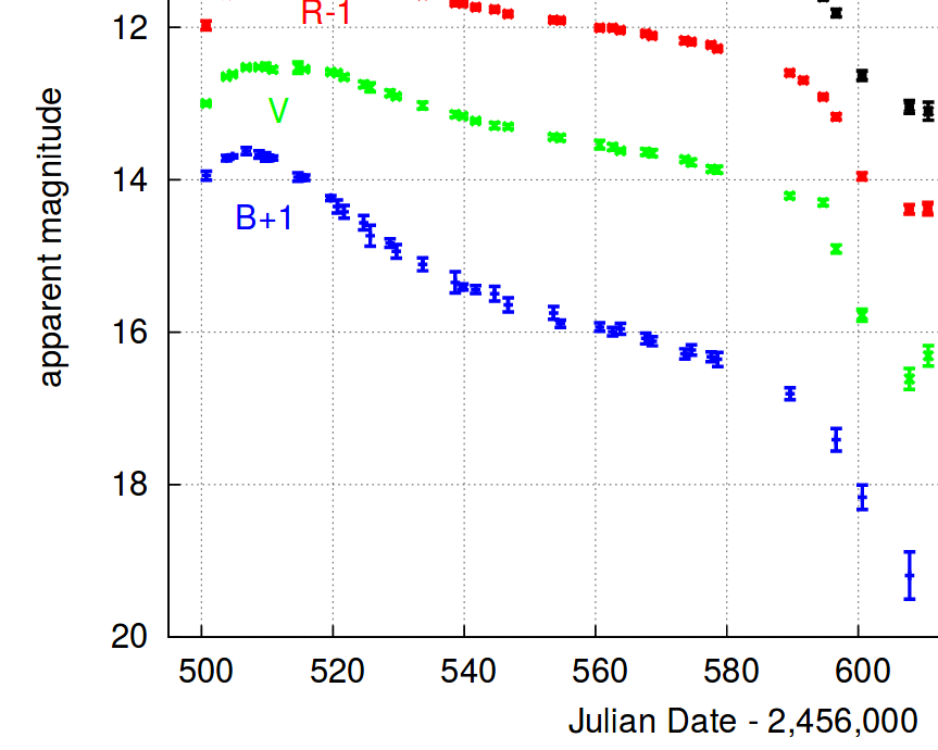
As an example of this technique, let's look at the nearby SN IIP 2013ej in M74. Its light curves show clear evidence for a "plateau" as the photosphere recedes into the ejecta.
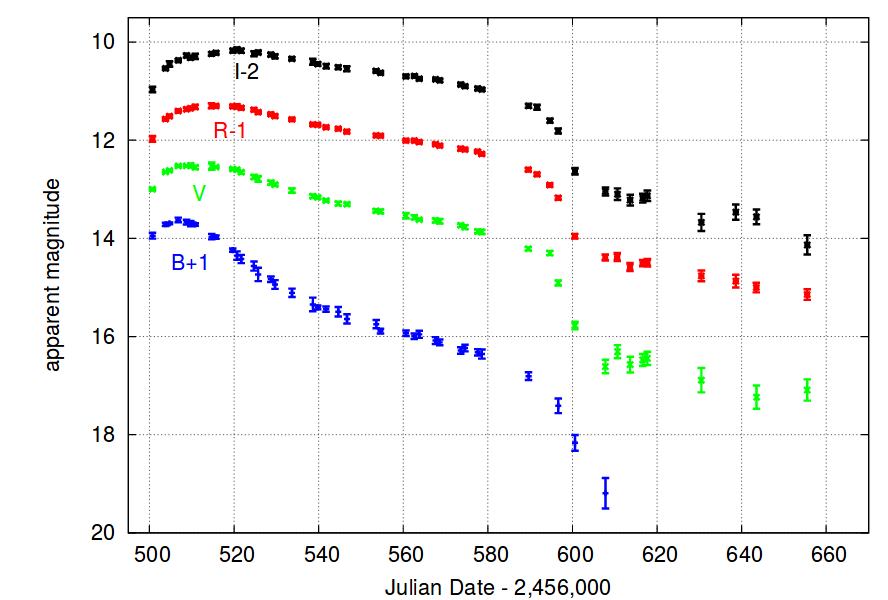
Figure 3 of
Richmond, JAVSO 42, 333 (2014)
We'll use only the V-band measurements for this quick little in-class calculation. Let's pick the date JD = 2456510, which is just a bit after the time of maximum light.
  Q:  Step 1: What is the apparent V-band magnitude of
        this SN on the date 2,456,510?
Taken from Figure 3 of
Richmond, JAVSO 42, 333 (2014)
If one assumes that the photosphere is emitting like a blackbody, then one can estimate the temperature by fitting the measured fluxes to spectra of Planck functions for different temperatures. The temperature will decrease with time, in general.
  Q:  Step 2: What is the temperature of the photosphere of
        this SN on the date 2,456,510?
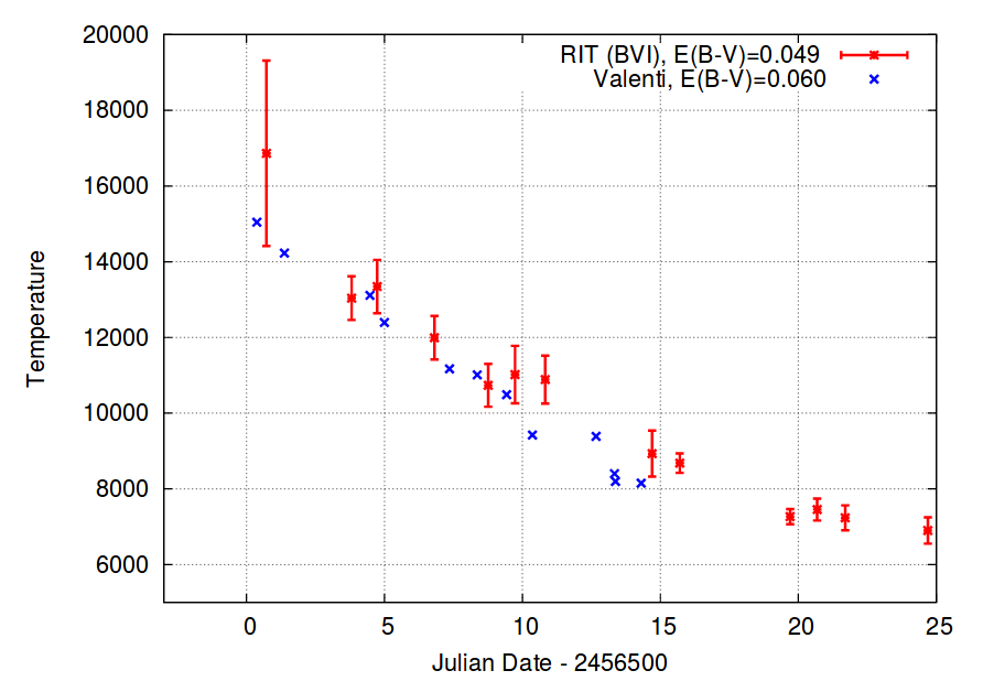
Taken from Figure 8 of
Richmond, JAVSO 42, 333 (2014)
We'll need to know the velocity of this portion of the ejecta in order to figure out its size. Observations and modelling by a number of researchers suggests that the explosion occurred on JD 2,456,494, so our chosen date of 2,456,510 is about 16 days after explosion.
  Q:  Step 3: What is the velocity of the photosphere of
        this SN on the date 2,456,510?

        (perhaps lines of hydrogen are best ...)
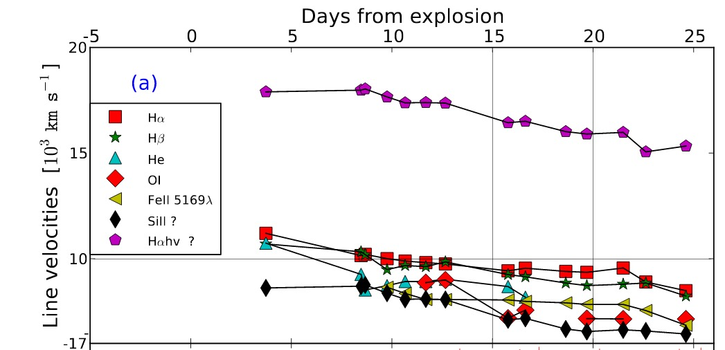
Figure 2a modified slightly from
Valenti et al., MNRAS 438, L101 (2014)
I'll provide the following handy facts to help you:
So, you should now be able to make a rough guess at the distance to this supernova.
   a)  Compute the size of the photosphere on the date 2,456,510.

   b)  Assuming a blackbody spectrum, calculate the total
             luminosity at all wavelengths

   c)  Calculate the luminosity emitted in the V-band only

   d)  Calculate the flux observed in V-band at Earth on the
             date 2,456,510

   e)  Use the inverse square law to compute the distance (in Mpc)
When I went through a more complicated procedure using data from this supernova, I found that the Expanding Photosphere Method yielded a distance of about 9.1 +/- 0.4 Mpc. Other methods suggest a similar distance. How does your value compare?
EPM has some weaknesses and strengths:
We can apply this technique to large distances, because Type IIP SNe are very luminous: their typical absolute magntiudes are between -15 and -18. Look at the example of SN 2013eq!
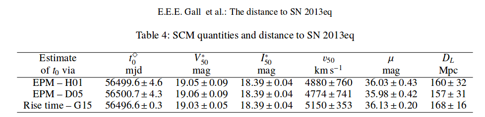
Table 4 taken from
Gall et al., A&A 592, 129 (2016)
Now let's consider the "White Dwarf" supernovae. The basic idea for using them as distance indicators is very simple:
Many (but not all) Type Ia SNe tell us their relative luminosity
In the Old Days (1970s and 1980s), the collection of measurements was relatively small and inhomogeneous. At that time, it seemed possible -- within the uncertainties -- that all Type Ia SNe had the same absolute luminosity; in other words, it seemed possible that they might be standard candles.
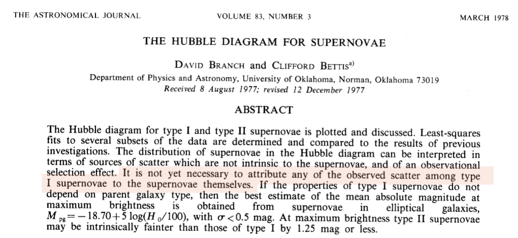
Abstract from
Branch and Bettis, AJ 83, 224 (1978)
However, as astronomers accumulated better measurements and larger samples, it became clear that SNe Ia are not all identical. These supernovae appear to vary in a systematic way.
For example, if we measure the amount by which supernovae decline in brightness 15 days after maximum light in the B-band,
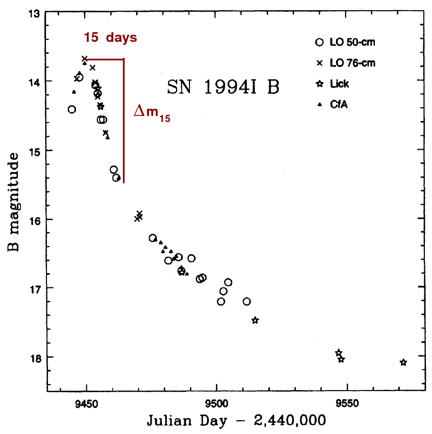
Figure taken from
Richmond et al., AJ 111, 327 (1996)
and compare it to the absolute magnitude of the event, we find a clear correlation.
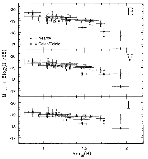
Figure taken from
Hamuy et al., AJ 112, 2391 (1996)
    Superluminous        Normal          Subluminous
 -----------------------------------------------------

     decline slowly                     decline quickly

     bluer                              redder

     faster ejecta                      slower ejecta

 -----------------------------------------------------
If we can measure enough SNe Ia to pin down these relationships between absolute magnitude and other observable quantities, we can perhaps turn SNe Ia into standard-izable candles; not as nice as truly standard candles, but still useful. There are several groups working on this problem, with slightly different techniques, and both have found some success. The SALT procedure involves choosing one of a set of templates which best fits the light curve of some particular observed SN Ia.
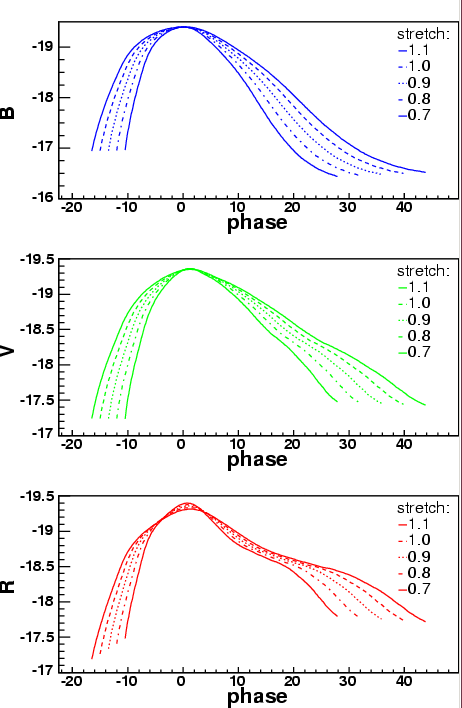
Figure taken from
Guy et al., A&A 443, 781 (2005)
Using these methods to correct for the relationship between decline rate and luminosity, one can reduce the uncertainty in distance modulus measurements for SNe Ia to perhaps 0.15 magnitudes.
  Q:  If the uncertainty in distance modulus
      is +/- 0.15 magnitudes, what is the
      uncertainty in distance?

      Express as a percentage.
If one looks at SNe in the near-infrared H-band, they may indeed be nearly identical; the Hubble diagram below uses measurements which have NOT been corrected for the decline-rate effect. To be fair, much less work has been done in the near-IR than in the optical.
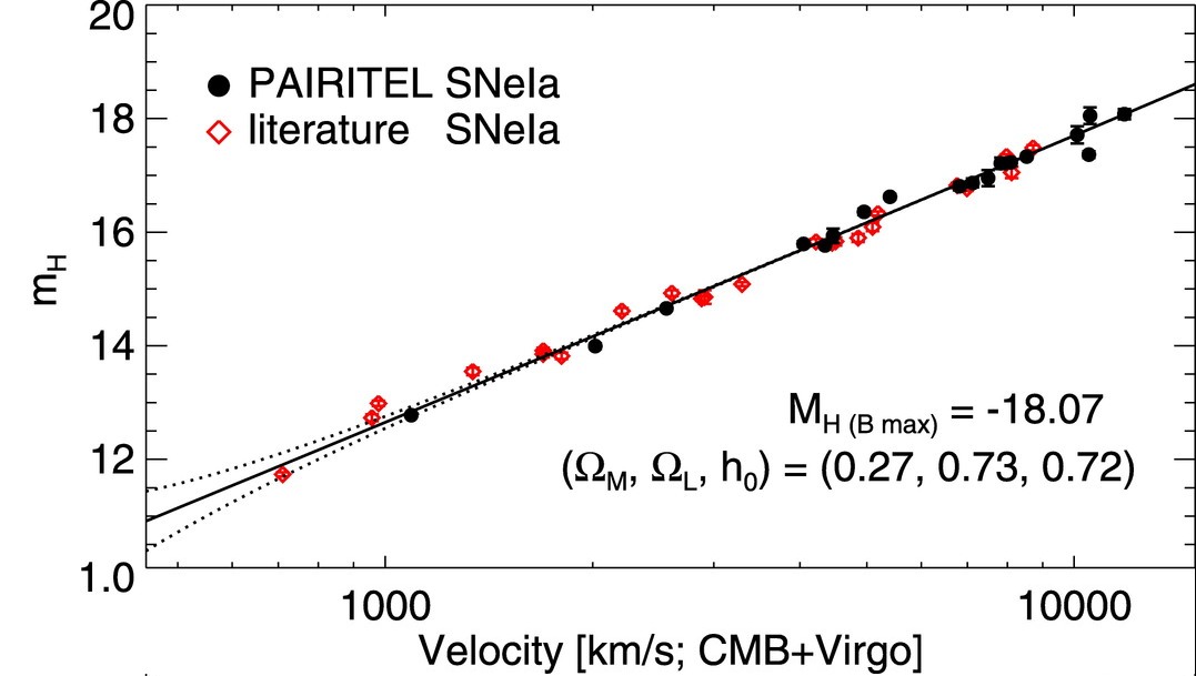
Figure taken from
Wood-Vasey et al., ApJ 689, 377 (2008)
One of the reasons astronomers spend so much time trying to understand Type Ia SNe is that they are really, really luminous: their absolute magnitudes are around -19 or -20! That means that they can be seen at VERY large distances, which means that they may be able to test different cosmological models.
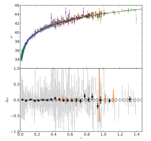
Figure taken from
Amanullah et al., ApJ 716, 712 (2010)
  Q:  What is the largest redshift out to which
      SNe Ia have been detected, as shown in
      the figure above?


      What is the distance modulus to that
      location?  Just look at vertical axis.


      To what (luminosity) distance, in Mpc, does that
      correspond?

         If you have a network device,
         go to Ned Wright's Cosmology Calculator
         and look it up.

         If you don't, use the definition
         of distance modulus.
Let's give it a try! Our target will be SN 2011fe in M101, which is one of the "good" Type Ia supernovae for distance measurements:
A portion of the B-band light curve measured by Richmond and Smith, JAVSO 40, 872 (2012) is shown in the figure below.
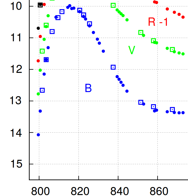
  Q:  What is the apparent B-band magnitude at peak?

  Q:  What is the Δm15 value in the B-band?

  Q:  Use the  relationship between decline rate and absolute magnitude
         as quantified by  Prieto, Rest and Suntzeff, ApJ 647 (2006)

                 MB = -19.325 + 0.636 ( Δm15 - 1.1)

         to compute the absolute B-band magnitude of this event.

  Q:  Compute the distance to this galaxy.
You can compare your distance to those derived using other techniques:
Now, one last word on Type Ia SNe: even the "good" events only provide relative distances. If we account for the relationship between decline rate and luminosity, we can determine the distance of one SN to another --- but we need to know the absolute distance to the first SN to turn these ratios of distance into Mpc. This makes Type Ia SNe one of the "secondary" distance indicators; or, more accurately, a "tertiary" indicator. The problem is these explosions are so uncommon that we haven't seen many (or any) in regions of space close enough to be reached with parallax, or even with some other methods. So we need at least 3 steps:
Still, even with this caveat, type Ia supernovae provide a powerful tool, because we can see them (and measure their properties) SO FAR AWAY!
Copyright © Michael Richmond.
This work is licensed under a Creative Commons License.
_male_(13994461256).jpg)