 Copyright © Michael Richmond.
This work is licensed under a Creative Commons License.
Copyright © Michael Richmond.
This work is licensed under a Creative Commons License.
We need to find new methods to reach out father into space, well beyond the Milky Way Galaxy and outside the Local Group. If we wish to measure the distance to a galaxy in the Virgo Cluster, for example, we have to leave fundamental methods behind and start to adopt more indirect techniques.
As you will see, some of the methods described here are called "secondary distance indicators" because we
These methods are not as secure as the direct ones --- they make our ladder begin to tilt and sway. But sometimes, these secondary methods are the best we can do.
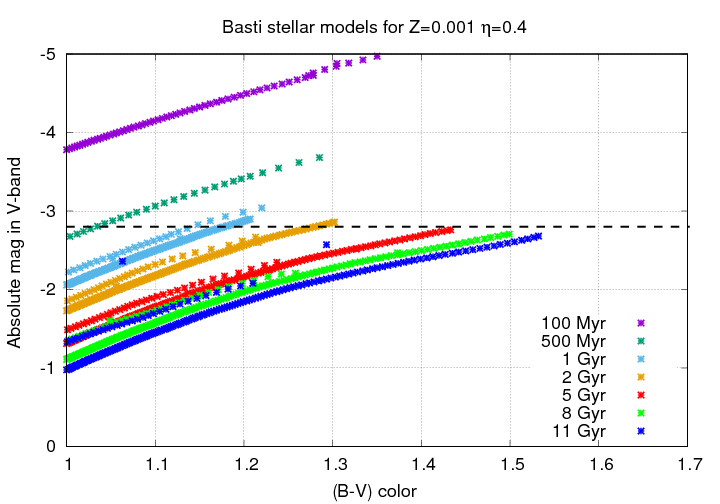
Let's look at the HR diagram of a group of stars, all born at the same time, with identical chemical compositions. I'll choose a metal-poor population, with
This should be relatively typical of an old stellar population, like that in the halo of our Milky Way, or the halo of other galaxies.
To make models of stars as they evolve, I'll use the
Let's begin with very young stellar populations. The figure below shows the HR diagrams for clusters of stars with ages of 100 and 500 Myr.
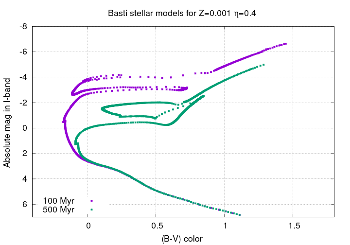
  Q:  What changes do you see between 100 and 500 Myr?


  Q:  What happens to the magnitude of the most
      luminous red giants as the cluster ages?
Now, as time passes, the stars continue to evolve ... but the rate of change decreases. This is simply a result of the longer lifetimes and slower evolution of the lower-mass stars which remain.
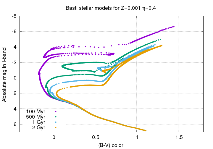
But not only does the pace of change slow down -- something rather peculiar, but very, very useful for astronomers, is happening at the tip of the red giant branch.
  Q:  What happens to the tip of the red giant branch
      between 1 Gyr and 2 Gyr?
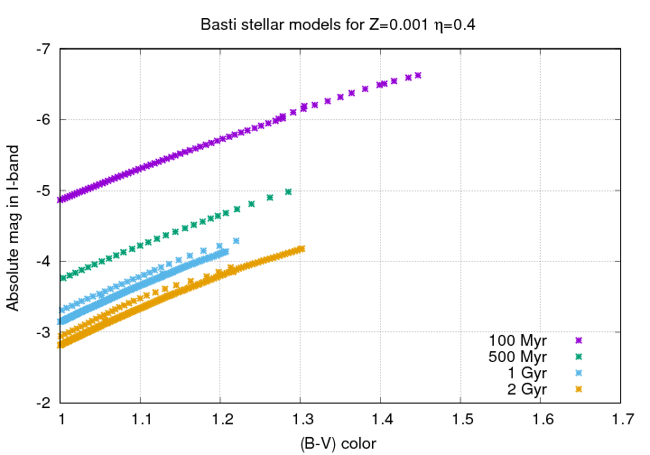
Let's zoom in on this region. One thing you'll notice is a set of parallel tracks for the stars of each age. In those cases, the lower, more solid track shows stars of slightly lower mass, which are just ascending the red giant branch (RGB) for the first time, and then starting to descend it; the upper, more sparse track shows stars of slightly higher mass, which are making a second journey up the red giant branch before they leave for good (probably turning into planetary nebulae). The track of those making their second trip is sometimes called the Asymptotic Giant Branch (AGB).
If we look at even older groups of stars, we will see that this tip of the RGB becomes redder .... but remains roughly the same luminosity.
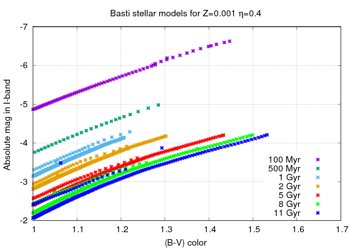
The absolute magnitude of this Tip of the Red Giant Branch is nearly constant from 5, to 8, to 11 Gyr.

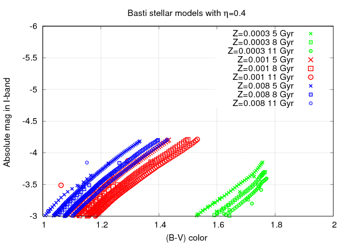
Now, I've cheated just a little bit. If you look closely, you'll see that on the y-axis of these graphs, I've put the "absolute magnitude in I-band," rather than the more common "absolute magnitude in V-band." It turns out that in the V-band, the absolute magnitude of this tip does change a bit more strongly, growing fainter as time passes:
Astronomers have examined the possibilities, and it seems that the I-band is just the wavelength at which these red giants of different ages appear to have about the same luminosity. I don't know exactly why that it, but it's certainly convenient for us ground-based observers!
Of course, it's not perfect. If we look at models with different metallicities, we see that there IS some variation in the level of the TRGB, but only for very metal-poor populations.
This method was first described back in 1993
but it has been developed and extended over the past two decades. A good recent article is
which I'll use as a source for the following material.
The basic idea is pretty simple:
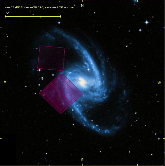
Here's an example. The galaxy NGC 1365 is relatively nearby, so we can resolve individual stars with HST. The purple squares mark the location of some images taken by HST in 2013.
Here's a copy of one of those HST images, which you can grab for yourself from the Hubble Legacy Archive. Let's zoom in one small region, away from the spiral arms:
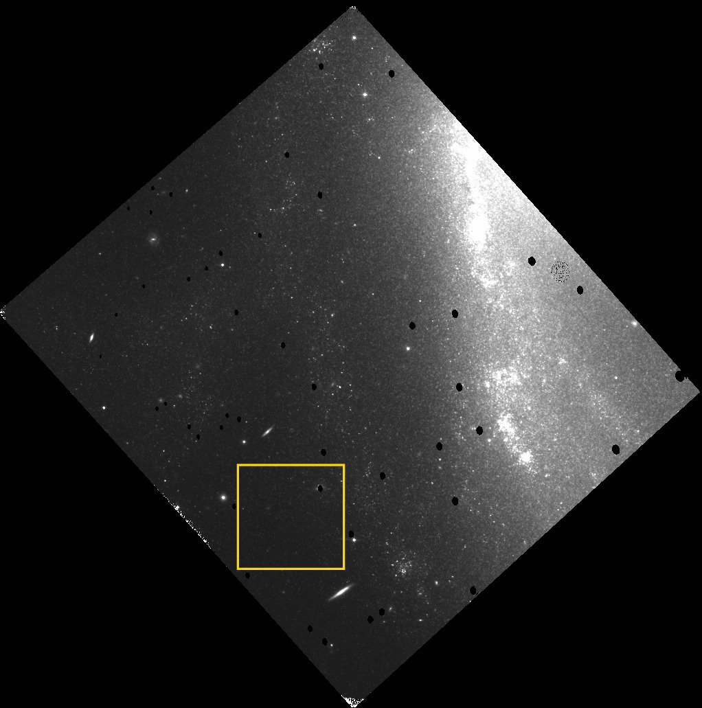
If we set the image contrast so that it shows only the very brightest objects ... we don't see very many.
But if we lower the threshold, a few more stars appear.
Lowering the threshold further makes a few more stars appear ...
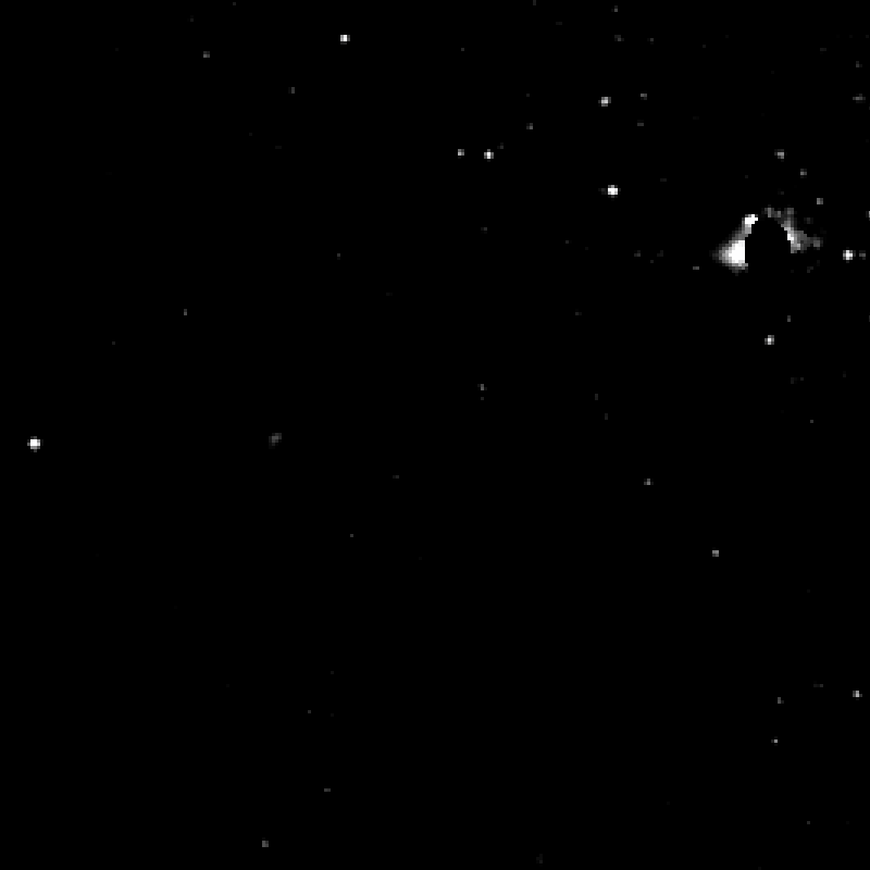
... but when we reach a certain point, suddenly a WHOLE BUNCH of stars appear, all at once. We have finally reached the level of the TRGB. (Click the image below to animate the sequence)
Now, let's look at how Jang et al., arXiv:1703.10616 put this into a quantitative form. They begin by making a color-magnitude diagram of stars in the images:
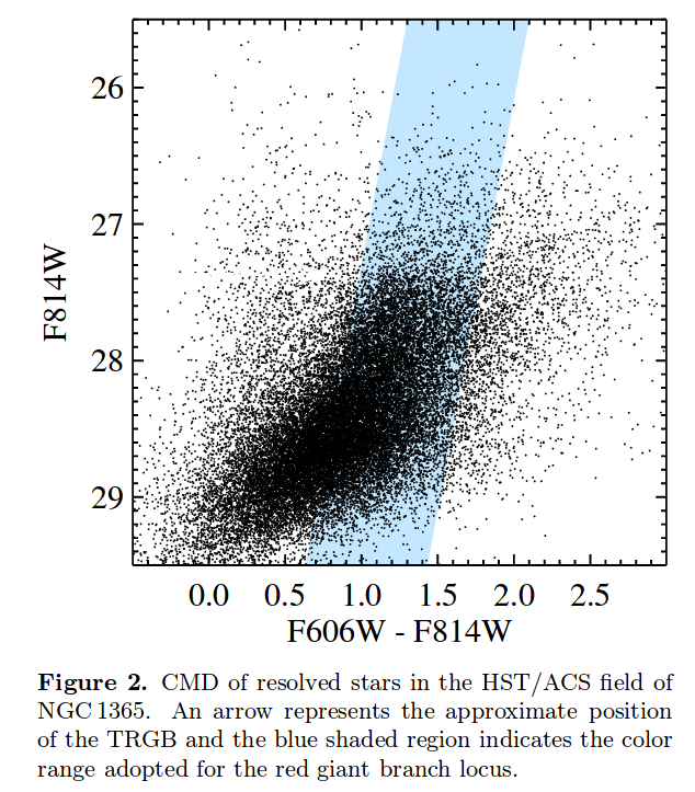
Figure 2 taken from
Jang et al., arXiv:1703.10616
and slightly modified.
  Q: Based on this CMD, what is the apparent magnitude
     of the TRGB?


  Q: Using that apparent magnitude, and absolute magnitude
     MI = -3.95  for the TRGB,
     what is the distance to NGC 1365?
The authors make a histogram of number of stars as a function of magnitude, smooth that histogram, and finally apply a matched filter to find the precise value at which stars suddenly increase in number.
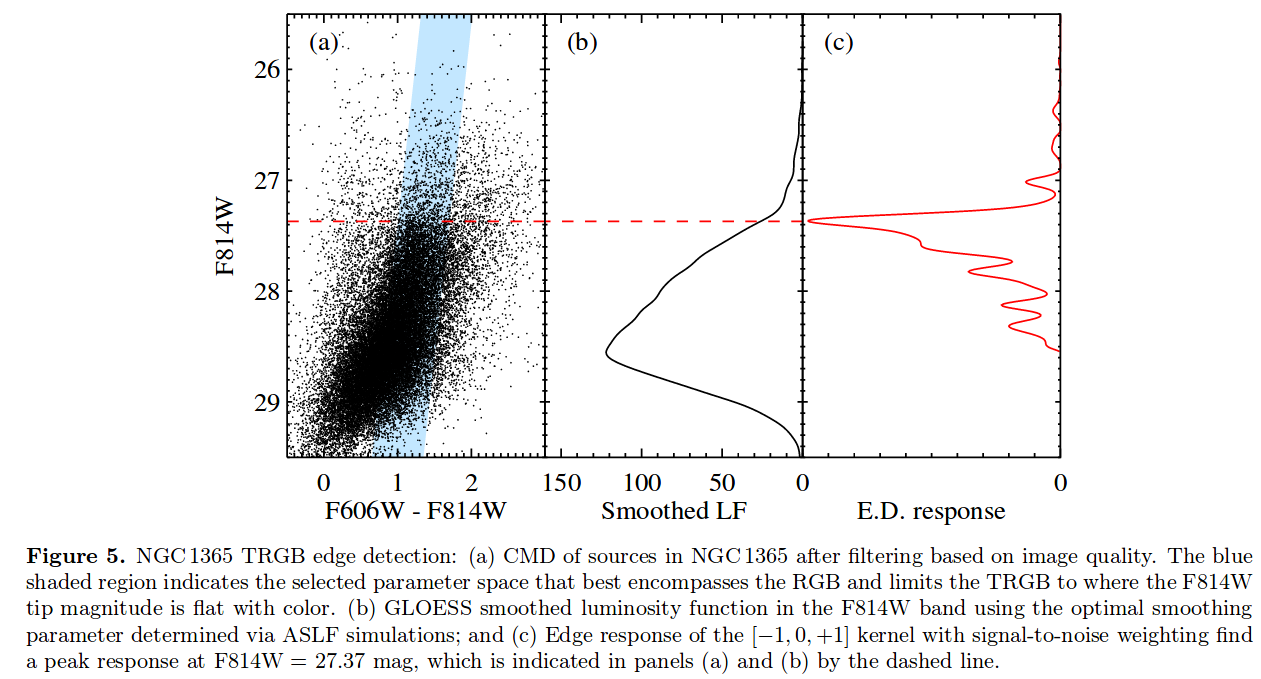
Figure 5 taken from
Jang et al., arXiv:1703.10616
They include a correction for a small amount of extinction, and end up with a distance to NGC 1365 of 18.1 Mpc:
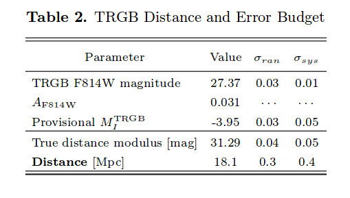
TAble 2 taken from
Jang et al., arXiv:1703.10616
The next technique is a little bit like TRGB, because it depends upon the fact that old stellar populations in different galaxies have similar properties. Instead of looking only at the very brightest red giants, however, this method includes all the bright red giants in a galaxy, together.
Imagine a very simple galaxy, in which all stars are identical: one mass, one color, one luminosity. We place this galaxy close to our Milky Way, at a distance of 10 Mpc, but not close enough to separate each star from its neighbors. Instead, we end up with a small number of these star blend together into each pixel.

With only a few stars in each pixel, the random fluctuations from one pixel to the next are pretty big: having one more star, or two fewer stars, is a big change from the average number. Therefore, we'll measure a large average fluctuation from one pixel to the next; in this case, 45 percent.
Now, suppose we move this galaxy twice as far away, to a distance of 20 Mpc. If we observe it with the same telescope, each of the pixels will now include a larger number of stars -- simply due to the larger physical area subtended at this larger distance. The average number of stars in each pixel will now be (2 x 2 = 4) four times larger it was originally.

If we again compare the number of stars falling into each pixel, we will again see random fluctuations -- but the size of these fluctuations will now be smaller relative to the mean than they were before.

   Q:  Can you fill in the blanks, computing the
       difference in each pixel from the mean value?


   Q:  What is the size of this difference from
       the mean value?
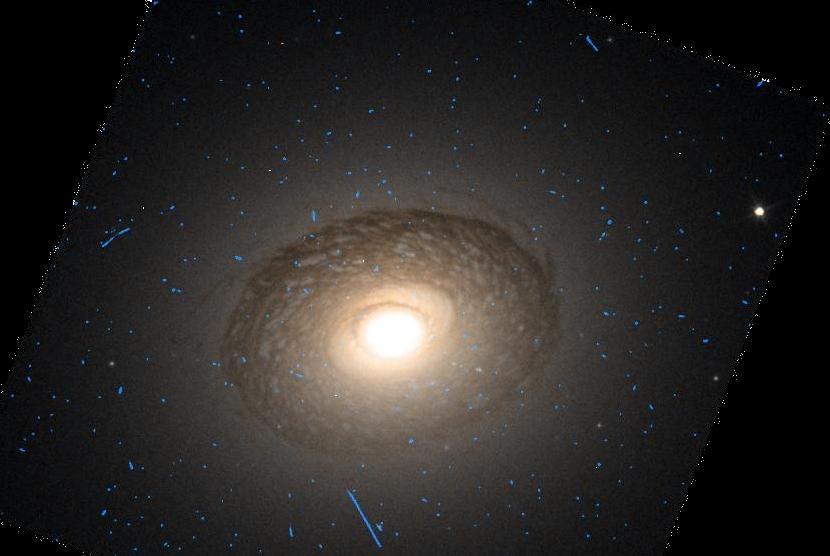
Let's look at a real example, taken from Blakeslee, Ap&SS 341, 179 (2012). HST observations of the galaxy IC 3032 in the Virgo Cluster show a pretty typical elliptical: bright at the center, fading away at larger distances:

Taken from Fig 7 of
Blakeslee, Ap&SS 341, 179 (2012).
If one makes a model of the galaxy's brightness, fits it to the distribution of light in the image, and subtracts it from the original, one is left with ... lumps. (Click on the image to activate animation)
Adapted from Fig 7 of
Blakeslee, Ap&SS 341, 179 (2012).
Those lumps are NOT individual stars in the galaxy; for one thing, they are much brighter than even the brightest red giants at this distance. Instead, they are due to Surface Brightness Fluctuations (SBF) in the number of bright giant stars falling within each resolution element of the image.
Now, real life is much more complicated than that simple example.
So the basic ASSUMPTION that the stellar census in old populations of all galaxies is identical has to be modified. Astronomers who use the SBF method must try to account for variations in the population of stars from one galaxy to the next. It's a very complicated business.
But the basic idea remains the same:
Large fluctuations means the galaxy is nearby; small fluctuations means the galaxy is far away.
This method works best at long wavelengths, in the optical I-band and in the near-infrared, because emission from a galaxy at those wavelengths is dominated by a relatively few, luminous, red giant stars. If we observe at shorter wavelengths, then we dilute the light of these few, luminous giants with the light from many more less-luminous subgiants and main-sequence stars. That means that the number of stars contributing to the light inside each pixel (or resolution element) increases, and the size of random fluctuations in that light will decrease.
Two reasons the SBF method is so promising are
The reach of the SBF method is larger than that of other methods we have examined so far. Although the results are still somewhat preliminary, it appears that SBF can be used to measure distances to the Coma Cluster of galaxies -- which it finds to be about 95 Mpc away from us, roughly six times more distant the the main Virgo Cluster!
The figures below are taken from a poster published in 2015, not from a refereed paper, so please consider them preliminary. Another poster was shown in Jan 2017, but the SBF group has still not published a paper on this object.
First, a near-IR image of the galaxy NGC 4874 taken with HST at 1.6 microns (in H-band):

Taken from
Jensen et al., "The Surface Brightness Fluctuation Distance to the Coma Cluster" (2015)
Now, the same image after subtracting a model for the galaxy's light, leaving surface brightness fluctuations and a boatload of globular clusters.

Taken from
Jensen et al., "The Surface Brightness Fluctuation Distance to the Coma Cluster" (2015)
The methods we've discussed so far today are not as mathematically sound as trigonometric parallax, but they don't rely on THAT many assumptions.
But our final topic today is one which involves more assumptions, including some which are very poorly understood. When we try to apply the Globular Cluster Luminosity Function method, we will have to fall back upon a somewhat weak argument:
I don't quite understand how globular clusters form, or why they have a particular distribution of luminosities ... but I am going to ASSUME that the clusters around galaxy A have the same distribution as those around galaxy B
We will simple assume that if two groups of objects have a similar appearance, that their properties must be the same in detail. It's quite a step away from individual stars, for which we can work out the physics in detail, or even a population of many stars.
Okay, enough philosophy. Back to science.
Globular clusters are collections of 10,000 to 1,000,000 stars orbiting within a compact space of a few parsecs. The stars within them belong to very old populations; in some cases, it appears that they may date from the time of our Galaxy's formation, or even earlier.
When we look at globular clusters within our own Milky Way, we can see very clearly the individual stars (except when they get in each other's way near the center, perhaps).
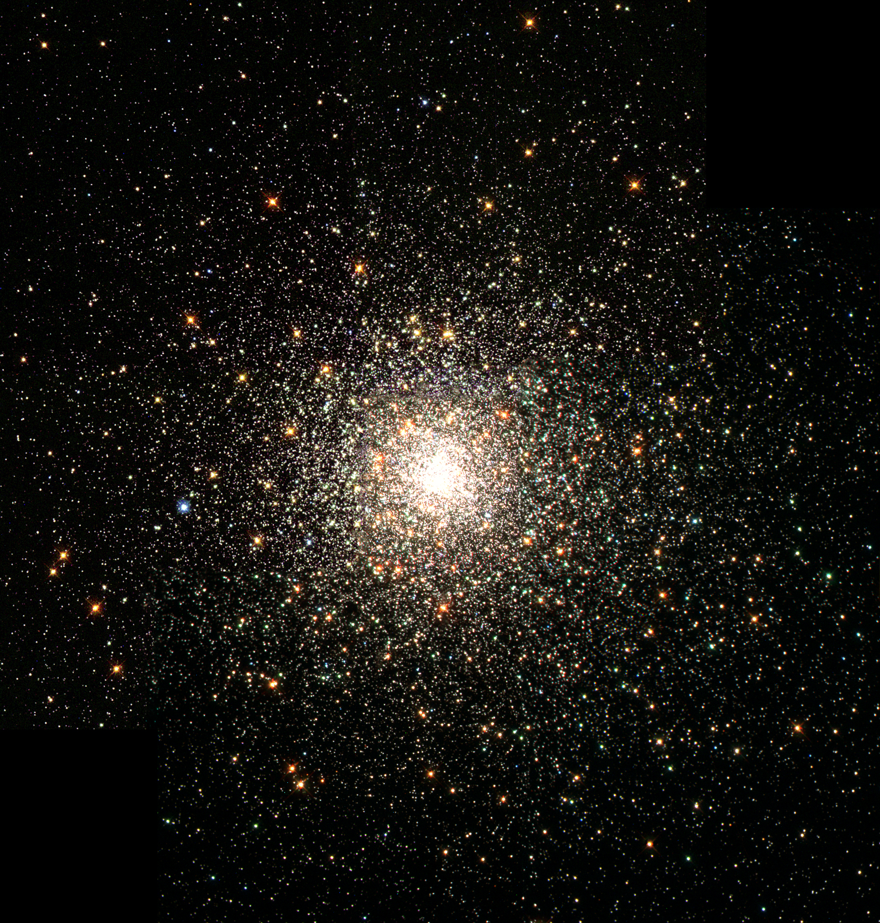
Image of M80 courtesy of
NASA and
Wikipedia
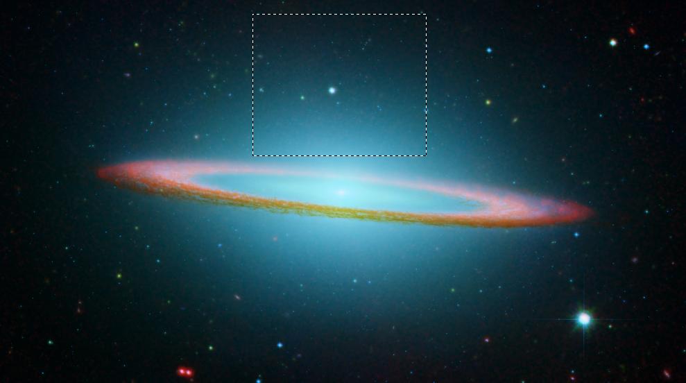
When we look at other galaxies, we can't resolve the individual stars; instead, we just see a compact, bright ball of light. In this picture of the Sombrero Galaxy, for example, note the many, many little dots which appear blueish in color.

Image of M104 from HST and Spitzer
courtesy of NASA/JPL-Caltech/University of Arizona
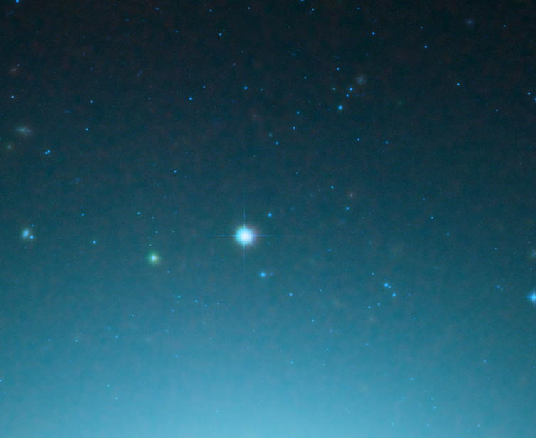
Here, I'll zoom in to show them more clearly.
Now, globular clusters are NOT identical: some are much larger than others, some are much more luminous than others. If we count the number of clusters in the Milky Way as a function of their absolute magnitudes, we find a roughly gaussian distribution. Yes, there's a tail at the low-luminosity end; no, for our purposes, that's not very important (why not?).
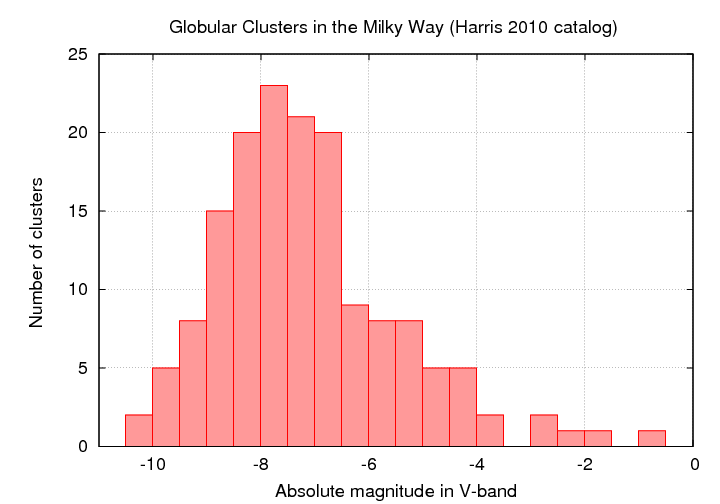
Figure based on data from
http://physwww.mcmaster.ca/~harris/mwgc.dat
If we look at the distribution of apparent magnitudes of globular clusters around other galaxies, we see something like a gaussian distribution (well, sometimes ... more on that in a moment). In the figure below, the left-hand panels show histograms of the GCs in a pair of Virgo Cluster galaxies.
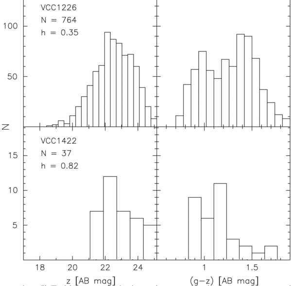
Figure taken from
Jordan et al., ApJS 180, 54 (2009)
The right-hand panels in the figure above show a histogram of the COLORS of the GCs around those two Virgo galaxies. It seems that GCs come in two flavors, "red" and "blue"; the difference has something to do with metallicity. Is the mixture of flavors the same in all galaxies? Does it matter for the use of GCLF as a distance indicator? Good questions.
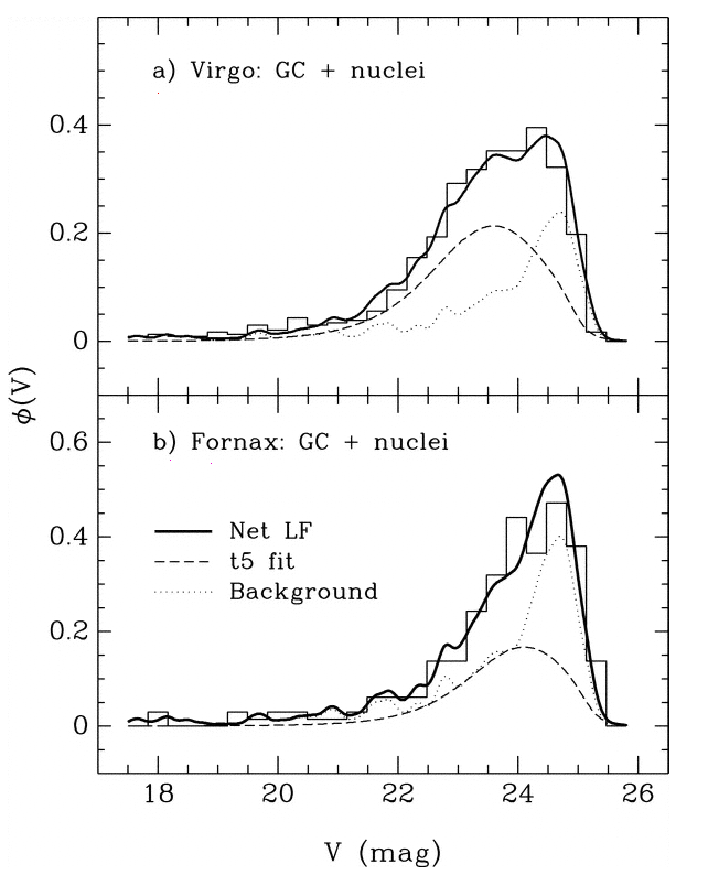
Figure taken from
Miller and Lotz, ApJ 670, 1074 (2007)
Let's put aside all these questions and just make the GIANT ASSUMPTION that the processes which formed globular clusters in the Milky Way also governed the formation of globular clusters around all other galaxies. In that case, the luminosity function for cluster around all galaxies should have the same absolute magnitude at its peak -- right? (Actually, in some cases, this might not be SO crazy -- see Harris et al., ApJ 797, 128 (2014))
  Q:  Choose either the Virgo or the Fornax
      distribution.  Compare it to the
      distribution of Milky Way GC absolute
      magnitudes.  Use it to estimate the
      distance to the Virgo or Fornax galaxy
      cluster.
If you have extra time, you might read about the dangers of incompleteness when one is comparing luminosity functions.
Copyright © Michael Richmond.
This work is licensed under a Creative Commons License.