 Copyright © Michael Richmond.
This work is licensed under a Creative Commons License.
Copyright © Michael Richmond.
This work is licensed under a Creative Commons License.
This is a small digression from our discussion of the globular cluster luminosity function (GCLF) method of measuring distances.
Let's go back and take a closer look at that last graph. It showed histograms of the observed luminosity functions of GCs in the Virgo and Fornax clusters. Concentrate on the lower panel. Is the model of the luminosity function, shown in the long dashed line, really symmetric?
Figure taken from
Miller and Lotz, ApJ 670, 1074 (2007)
No. It isn't symmetric. There are more clusters on the "bright" side of the apparent peak, and fewer clusters on the "faint" side.
  Q:  Why should the observed histogram show
      more clusters on the bright side of the peak?
The answer is pretty simple: bright objects are easier to detect! If you are looking for stars or clusters or galaxies or just about any sort of object in an astronomical image, you generally have a better chance of finding the bright items than the fainter ones. Pretty obvious, really.
The trouble is -- this introduces a systematic bias, or selection effect, into any analysis based on the detected objects. Depending on the particular sort of analysis, this sort of selection effect might be insignificant, or it might be very important.
  Q:  In this case, we are matching the peak
      apparent magnitude of the GCLF in Fornax
      to the peak absolute magnitude of the
      GCLF in the Milky Way.

      If we do NOT take the selection effect
      into account, what will happen to the
      distance modulus we compute?
Let's consider a second example. Suppose that we are interested in open star clusters, and we are making a catalog which contains the size of each cluster. We take a picture of the cluster Perseus 3 and see the pattern of stars below. The scale bar is marked in arcseconds.
Q: What is the radius of the cluster?
A few years later, another astronomer is granted time on a bigger telescope and takes a series of exposures of Perseus 3 with a range of exposure times. Click on the picture above to see the results of his work.
Q: What is the radius of the cluster?
So, how can we deal with this menace to quantitative measurements? We must counter-attack with a quantitative correction for the effects of the varying degree of completeness. What we need is a way to describe the probability that an object is detected as a function of its magnitude. Not as simple as
but more sophisticated, like this:
If someone else has studied this particular region of the sky with a bigger telescope some time in the past, and published a detailed catalog of the objects in the area, then we can compare that catalog to the objects in our study to make this sort of table.
Alas, in most cases, there is no pre-existing deep catalog of objects in the area which one is examining.
  Q:  How can we make any accurate statements
      about the probability of detection if don't
      really know what we ought to be seeing?
In the "old days", this was a tough problem. Since we have these newfangled devices called computers, however, there is a straightforward procedure we can follow to get a good, quantitative measure of incompleteness. The following Calvin and Hobbes comic strip may give you a clue ...
Start with some image showing the region of interest. This is a portion of the XMM-Newton/Subaru Deep Field.
Use some tool to find and measure the properties of all the objects in the image.
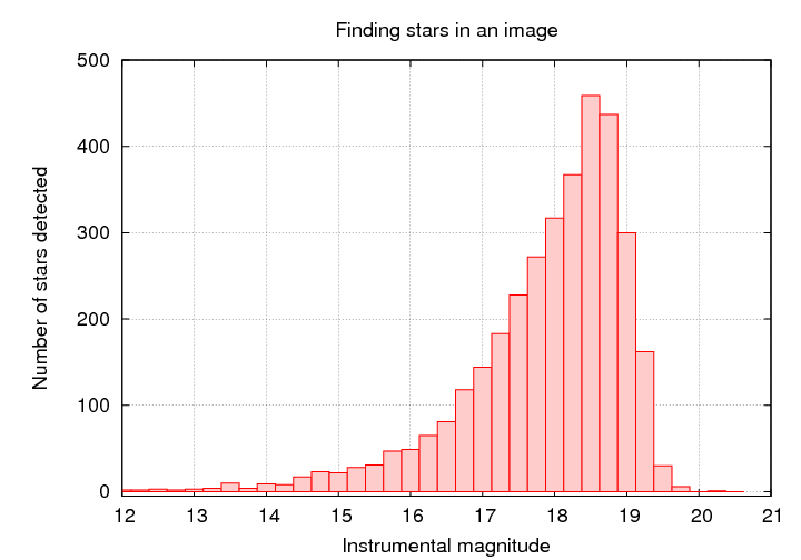
   Q:  At what magnitude do you think
       we fail to detect stars?
Now, the tricky part: use some tool to generate a set of fake objects, with the same size and shape as real objects, at random locations. Add those fake objects to the original image.
It's pretty easy to see the fake stars in the image above, isn't it? Try an image with fainter fake stars ...
Run this synthetic image, with real and fake objects, through your object-finding tool. Compare the list of objects found to the list of fake stars added. Compute the fraction of all the fake objects which were actually detected by your software.
Repeat for fake objects covering a wide range of magnitudes.
You can then make quantitative statements about the fraction of REAL objects which were (probably) detected by your software.

The point at which the fraction of objects detected falls to 50% is commonly used to define the completeness limit or plate limit. You must be very, very careful if you attempt to use measurements which are close to, or -- heavens above! -- beyond the completeness limit.
Fleming et al., AJ 109, 1044 provides a nice little analytic function which may work well to model the fraction of objects detected as a function of magnitude.
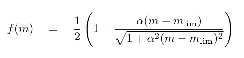
That function makes a gentle "sigmoid-ish" transition from 1.0 to 0.0 over a range which can be adjusted by the parameter α. It's similar to the shape seen in, for example, the case of stars in the XMM-Subaru Deep Survey.
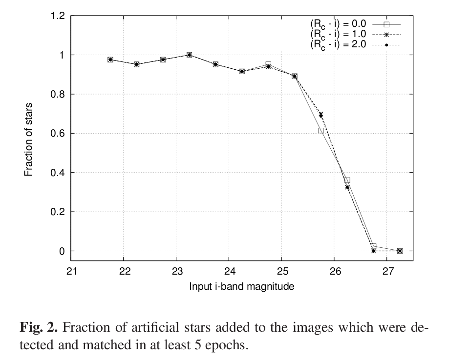
Figure taken from
Richmond et al., PASJ 62, 91 (2010)
Copyright © Michael Richmond.
This work is licensed under a Creative Commons License.