 Copyright © Michael Richmond.
This work is licensed under a Creative Commons License.
Copyright © Michael Richmond.
This work is licensed under a Creative Commons License.
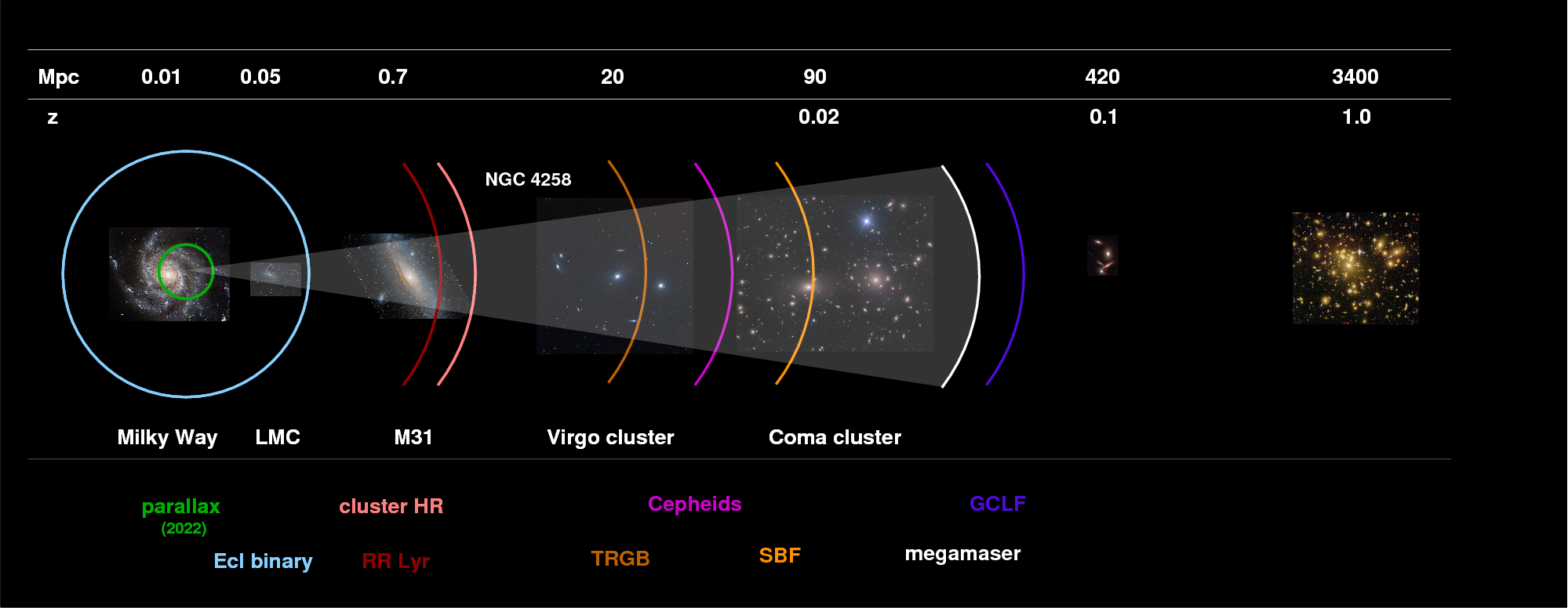
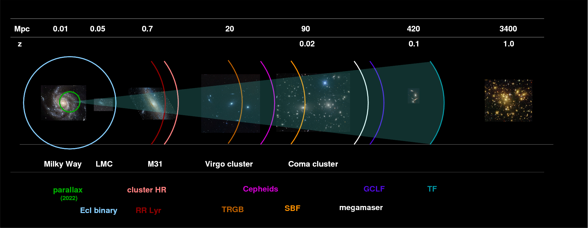
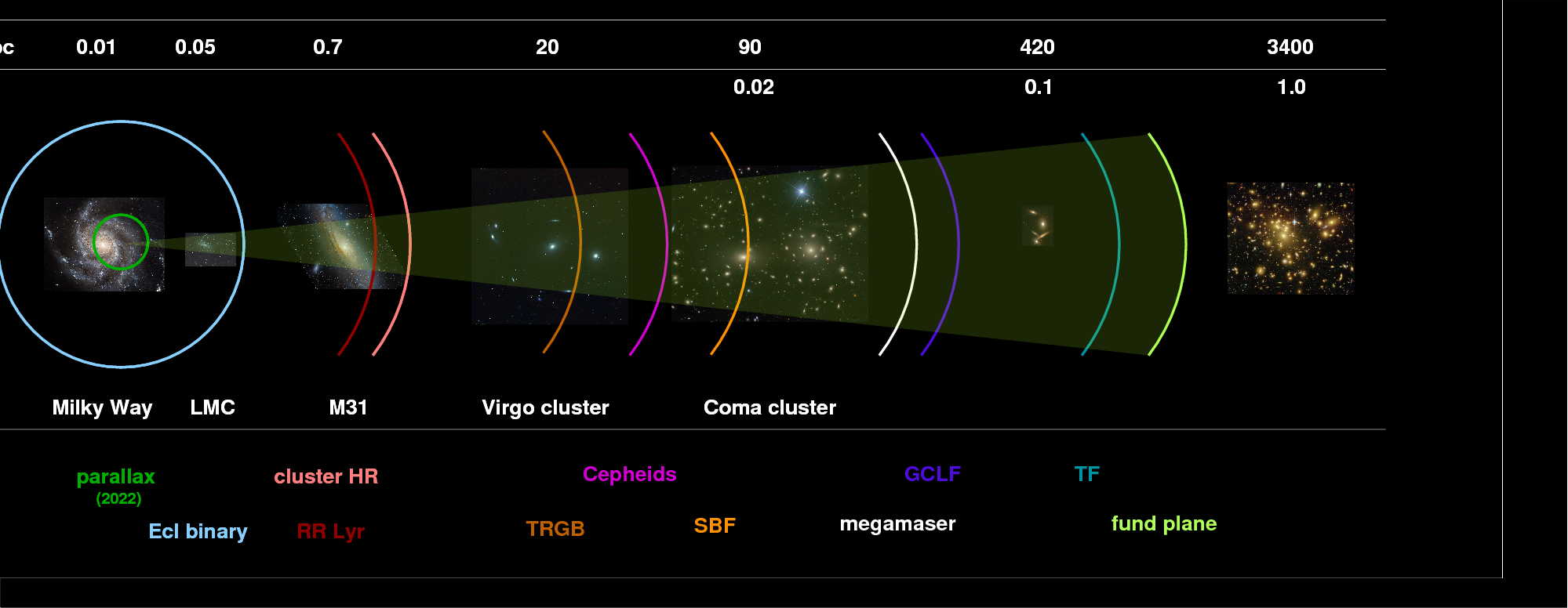
The methods we've described so far can only reach out to the nearest galaxy clusters. If we wish to probe deeper into the universe, we need to find new ways to estimate distances. The methods I'll describe today each have a strong point and a weakness.
The latter two methods are sometimes called "tertiary distance indicators" because they depend on at least two earlier steps of the distance ladder to calibrate them properly.
Let's concentrate on the most nearby and best-studied object in this category: NGC 4258. It looks like an ordinary spiral galaxy in the optical
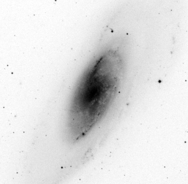
Image thanks to
the Aladin Sky Atlas
but X-ray and radio data indicate that there is a supermassive black hole at the center of the galaxy's bulge, making it an Active Galactic Nucleus (AGN). Now, lots of galaxies have AGN at their centers, but NGC 4258 is special: within the accretion disk of gas which orbits around the black hole at its center are certain clouds which have just the right combination of properties to create masers. In particular, water molecules making the transition 616-523 emit radiation at 22.235080 GHz.
The important point about these masers, from our point of view, is that they act like tiny little spotlights: they are bright enough that we can measure VERY precisely the
How precise are the measurements? Combining signals from a number of telescopes -- the Very Large Array (VLA) and the Very Long Baseline Array (VLBA), each of which consists of many dishes spread over a large areas, and the Effelsberg 100-m single-dish telescope -- yields positions better than 0.1 milliarcsec, and velocities good to about 1 km/sec. Only masers provide the strong, unresolved signals needed to reach such high precisions.
Here's what we see at the center of the galaxy at these radio wavelengths: a set of unresolved sources, redshifted on one side of the center and blueshifted on the other. The intensity of the color in the figure is related to velocity: the fastest blobs are deep red and deep purple.
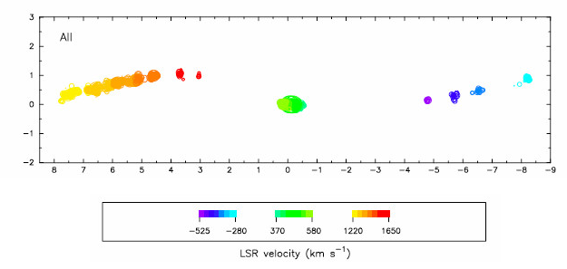
Figure taken from
Moran, ASP Conf Ser 395, 87 (2008)
   Q:  Look at the pattern of the masers.
       Does it look like the simple Keplerian
       motion of clouds in a simple ring?
No, it doesn't. If all the clouds were in a ring, at a single distance from the central black hole, then we ought to see the largest speeds in the outermost blobs; but the observations show the largest speeds in the INNERMOST blobs.
It turns out that the geometry is pretty complex, something like this:
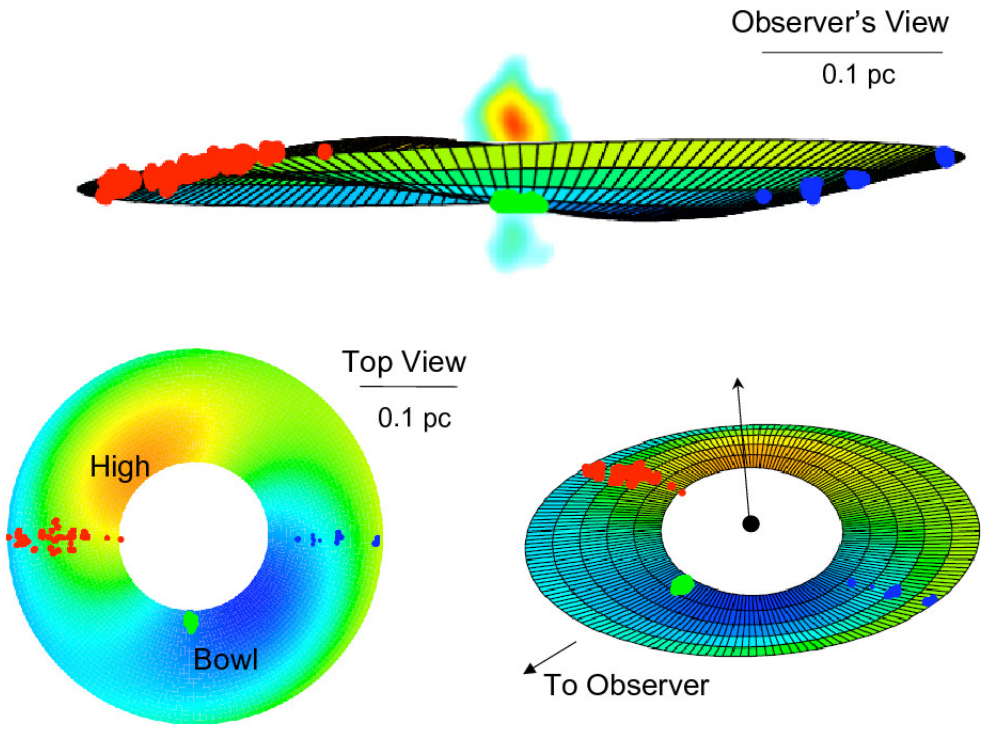
Figure taken from
Moran, ASP Conf Ser 395, 87 (2008)
The accretion disk is warped, and the masers we see are scattered throughout the disk, some much closer to the center than others.
But we can be pretty sure of several things:
and so
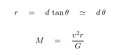
In other words, we can expect simple relationships between velocity v, orbital radius r, acceleration a, and the mass of the central black hole M:

Of course, we can't directly observe all these quantities; the only things we measure directly are the angular positions of the masers, relative to the central source, and their velocities.
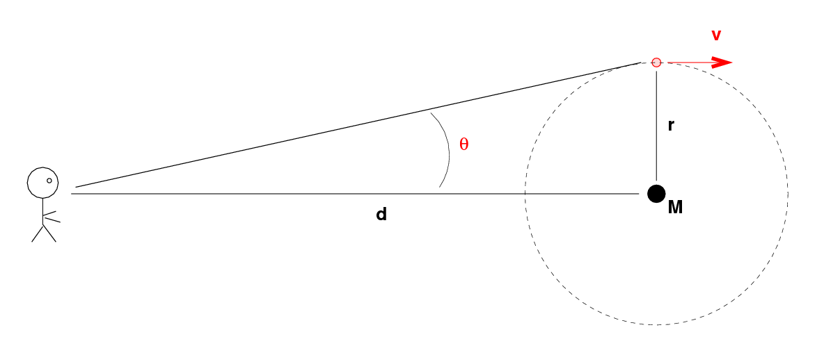
  Q:  Can we use the observed angle θ and radial velocity v
      to figure out the distance d?
Well, let's see ... IF we knew the distance d, then we could compute the orbital radius r and the mass of the central object M.
Let's play a little game. I'll choose one maser from the observed set, with the following properties:
    radial velocity      v  =   1000 km/sec           rel to center

    angular separation   θ  =   0.005 arcsec          from center
Each student will just GUESS a distance, and then use that distance to compute the orbital radius r and mass M of the black hole.
  distance d       orbital radius     central mass
    (Mpc)                r                M
--------------------------------------------------------------------------

     5              _________          __________         ___________


     7              _________          __________         ___________


    10              _________          __________         ___________


--------------------------------------------------------------------------
Hmmm. It seems that there is no unique solution: for any given distance, we can find an orbital radius and central mass which produce the observed quantities. In other words, we CANNOT determine the distance to NGC 4258 with this information alone. That should be no surprise. Both the orbital radius r and the central mass M depend linearly on the distance to the galaxy d.
But ... if we could find some observable quantity which had a DIFFERENT dependence on the distance, then we might be able to find a unique solution. Suppose we could measure the acceleration a of this little cloud of gas? Recall that the acceleration depends on the RECIPROCAL of the orbital radius
which means it also depends on the RECIPROCAL of the distance d to the galaxy. Aha! If we could observe the acceleration, we could break the degeneracy and solve for the distance to the galaxy.
Where should we look? Here are the locations of the masing clouds again, as observed by radio interferometers:
Figure taken from
Moran, ASP Conf Ser 395, 87 (2008)
  Q:  Which of these clouds might be the best choice
      to detect the acceleration?

      Why?
Just how big is this acceleration? Can we really measure it? Well, let's find out. Use your values to fill in the acceleration column of your table.
  distance d       orbital radius     central mass          acceleration
    (Mpc)                r                M                    m/s2
--------------------------------------------------------------------------
                           3                   7
     5              25 x 10  AU        2.8 x 10   solar      ___________

                          15                   37
                  3.7 x 10   m         5.6 x 10   kg


                           3                   7
     7              35 x 10  AU        3.9 x 10  solar       ___________

                          15                   37
                  5.2 x 10   m         7.9 x 10   kg


                           3                   7
    10              50 x 10  AU        5.6 x 10  solar       ___________

                          15                   37
                  7.5 x 10   m        11.2 x 10   kg


--------------------------------------------------------------------------
Those values seem really small. How could we measure such tiny accelerations? Well, the good thing about accelerations is that they can accumulate over time into large changes in velocity.
  Q:  Suppose we measure the velocity of one cloud now,
      and then again after one year has passed.

      How large would the change in velocity be?
Radio astronomers have patiently monitored this galaxy for many years, watching for exactly these expected changes in velocity of the individual clouds. Below is a small sample of their results; the numbers in the upper-right corner of each panel refer to the number of days since 1994 Apr 19. Each cloud is drawn in a different color to help you follow the evolution of its velocity.
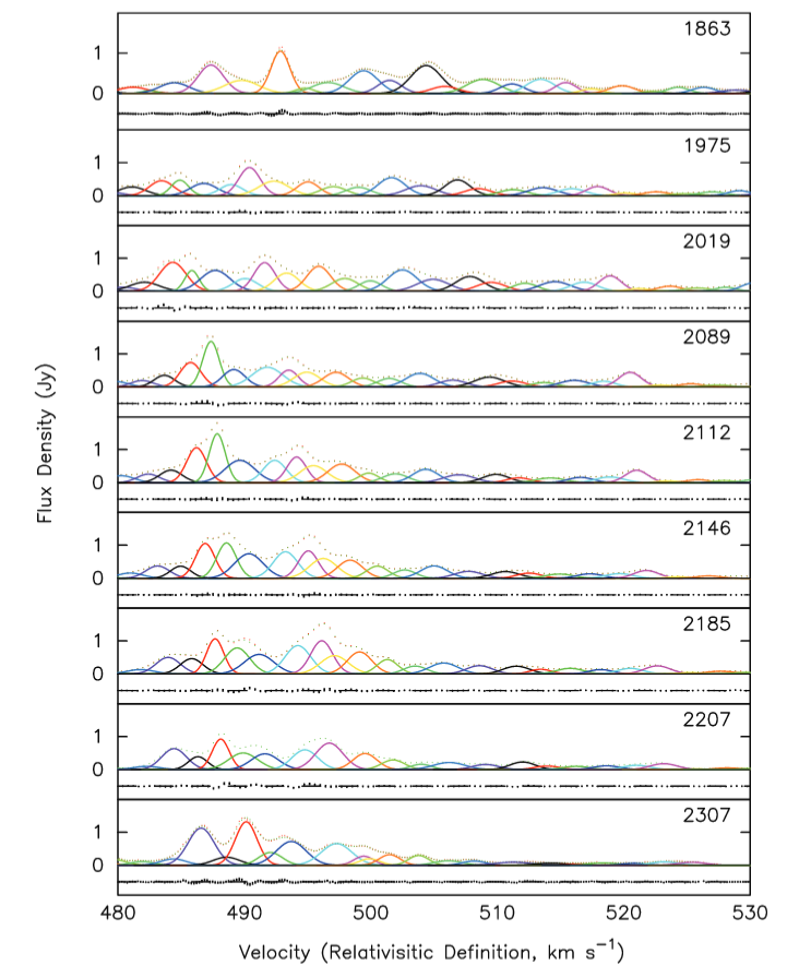
Modified from Figure 5 of
Humphreys et al., ApJ 672, 800 (2008)
Q: Pick one cloud and compute its acceleration.
So, as you can see, we CAN measure accelerations of the size produced by orbital motion around the central black hole. In theory, then, we can solve for the distance to the galaxy.
In practice, this is complicated because the clouds are all at different distances from the center, because the disk is not perfectly edge-on, and because it appears to be warped slightly. There are ... a number of parameters one must determine, not just the distance. But some astronomers have done all that work and conclude:
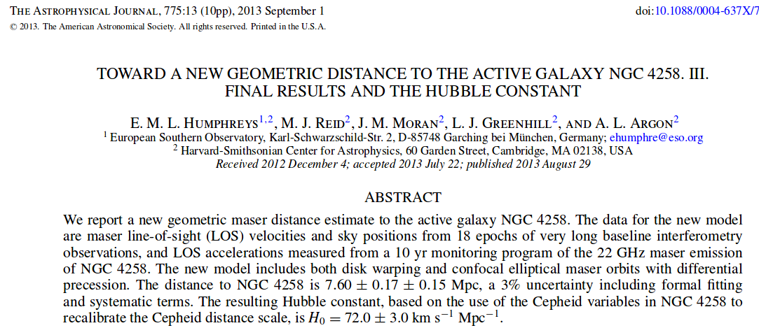
Abstract from
Humpheys et al., ApJ 775, 13 (2013),
just in case you couldn't figure it out for yourself.
The reason that I've spent so much time describing this one galaxy is that it provides a nearly geometric distance to an object far, far beyond the Milky Way. This distance does NOT depend on previous steps of the distance ladder (well, aside from the distance to the Sun). That means that we can use NGC 4258 to check our other methods of distance measurements -- at least, the methods that can reach it.
In addition, some radio astronomers are seeking out other examples of AGN with megamasers in their accretion disks, in order to use the same technique to measure their distances. The Megamaser Cosmology Project has published studies of five other galaxies, all much more distant than NGC 4258.
| Galaxy | Distance (Mpc) | Reference |
|---|---|---|
| NGC 3789 | 49.6 +/- 5.1 | Braatz et al., ApJ 718, 657 (2010) |
| NGC 6264 | 144 +/- 19 | Kuo et al., ApJ 767, 155 (2013) |
| NGC 6323 | 73 +26-22 | Kuo et al., ApJ 800, 26 (2015) |
| NGC 5765b | 126.3 +/- 11.6 | Gao et al., ApJ 817, 128 (2016) |
Although the number of objects we can measure with this method is very small, the DIRECT distances we can derive will serve as extremely valuable checks and calibrators of other techniques.
The key point of the Tully-Fisher relationship is that the speed of rotation of material in a spiral galaxy is related to the luminosity of that galaxy: high speeds occur in galaxies of high luminosity.
To establish this fact, Tully and Fisher, A&A 54, 661 (1977) (hereafter TF77 ) carefully selected galaxies for which rotation velocities could be measured accurately. They used radio telescopes tuned to the 21-cm line of neutral hydrogen, which is plentiful in the disks of many spirals. Gas is a very convenient tracer of dynamics because -- in ordinary spirals, at least -- it orbits the center of the galaxy in circular paths.
If one points a single-dish radio telescope at a typical galaxy -- as TF77 did -- the beam of the telescope is so large that it captures radio waves from the entire galaxy in a single pointing.

The radio image produced by an observation like this is bland: just a single unresolved blob of emission. However, one can easily measure the intensity of the radio waves at different frequencies, which corresponds to the amount of emission at different velocities within the galaxy. Here are eight examples from TF77, showing the measured radio intensity as a function of velocity.
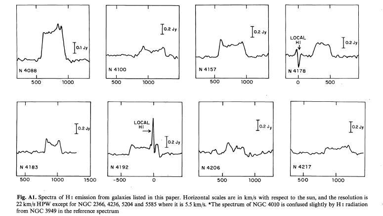
Figure A1 taken from
TF77
The measured width of the HI line needs to be corrected for the inclination of the galaxy: the more edge-on the galaxy, the smaller the correction. TF77 selected only galaxies with an inclination angle of at least 45 degrees, in order to minimize errors caused by this inclination correction. Notice the light tension here:
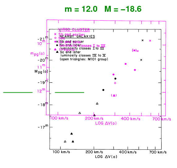
To calibrate their relationship, TF77 chose a set of galaxies which were close enough that astronomers had decent measurements of their distances; and, therefore, their luminosities (or absolute magnitudes). Unfortunately, this set didn't have very many high-luminosity systems. In order to test the relationship on high-luminosity systems, they observed galaxies in two nearby clusters, Virgo and Ursa Major. They didn't know the distance to those galaxies, but they could -- with some effort, as they describe in the paper -- find samples of objects which ought to be at the same distance, so that the apparent magnitudes would differ from the absolute magnitudes by a fixed offset.
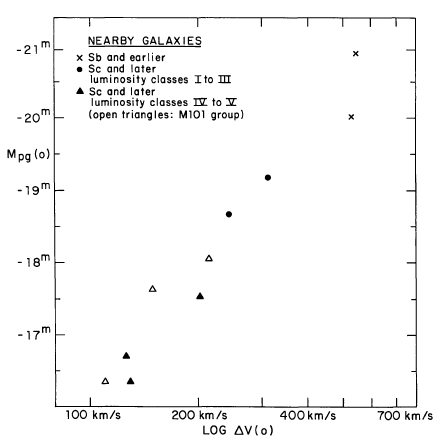
Fig 1 taken from
TF77
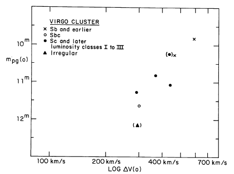
Fig 3 taken from
TF77
Now, the first question was -- is there a similar connection between rotational velocity and absolute magnitude for both groups of galaxies? Take a look for yourself in the figures above. TF77 concluded there was.
The second question was -- how can we USE this relationship? Well, if the connection is the same for all spiral galaxies, everywhere, then we should be able to determine the distance modulus (m - M) by simply sliding the data for the Virgo cluster galaxies until they line up with the results for galaxies with known absolute magnitudes.

  Q:  How much must one shift the Virgo Cluster galaxies
        in magnitude to make the match the nearby galaxies?


  Q:  What is the distance to the Virgo Cluster by this method?
If you wish, you can read a brief discussion of the term "luminosity class" when applied to a galaxy.
A good summary of recent work on the Tully-Fisher relationship can be found in Sakai et al. ApJ 529, 698 (2000) . The authors test the connection between HI velocity and luminosity in several different passbands, rather than the single bluish photographic passband of the earlier work. They find that the relationship grows tighter if one measures luminosity in the near-IR:
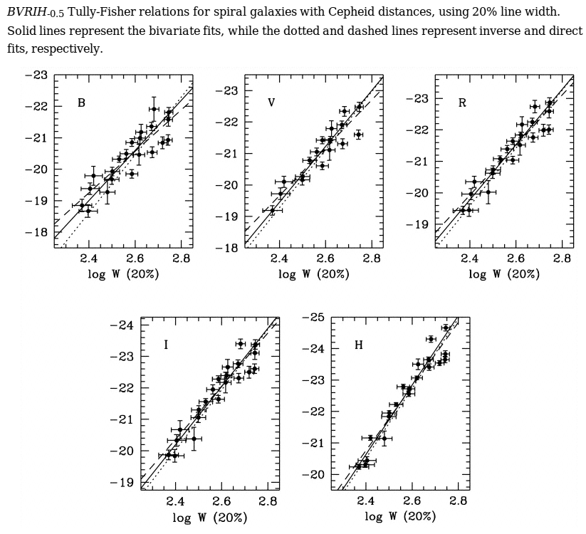
Figure 1 taken from
Sakai et al., ApJ 529, 698 (2000)
Note that TF77 found that the distance modulus to the Virgo cluster was (m - M) = 30.6 mag, or 13.2 +/- 1 Mpc; that agreed with the "short" value of the time, as opposed to the "long" value of (m - M) = 31.45 mag proposed by Sandage and Tamman. More recent work, such as Mei et al. ApJ 655, 144 (2007), finds a value somewhere in between, but closer to the "short" scale: (m - M) = 31.1 mag, or 16.5 Mpc. TF77 found the distance modulus to the Ursa Major cluster was (m - M) = 30.5 +/- 0.35 mag, or 12.6 +/- 2 Mpc. This is again a bit smaller than more recent values of (m - M) = 31.3 mag (Tully and Pierce ApJ 533, 744, 2000) or (m - M) = 31.6 mag (Watanabe et al. ApJ 555, 215, 2001).
How far away can one apply the Tully-Fisher method? Since all one needs to observe are the apparent magnitude of the entire galaxy (very easy), and the rotational velocity of objects in it (a bit harder), astronomers have tested it as far out as redshift z=1.4 (or many thousands of Mpc)! There are some complications at great distances, though:
But maybe worst of all
That last point could be a real killer. Imagine a galaxy in the early universe, at an age of perhaps 2 Gyr, with some mass M and rotational velocity v and luminosity L. If we look at that same galaxy in the current universe, at age 13 Gyr, it will have basically (unless there is some major merger) the same mass and same rotational velocity, but (probably) a very different luminosity L -- simply because some stars have disappeared, while others have formed.
So it's not surprising that one compares the properties of low-redshift and high-redshift samples, one can find some differences. As the figure below shows clearly, galaxies with the same rotational velocity at high redshift (filled black symbols) are considerably bluer than galaxies with the same rotational velocity at low redshift (open symbols).
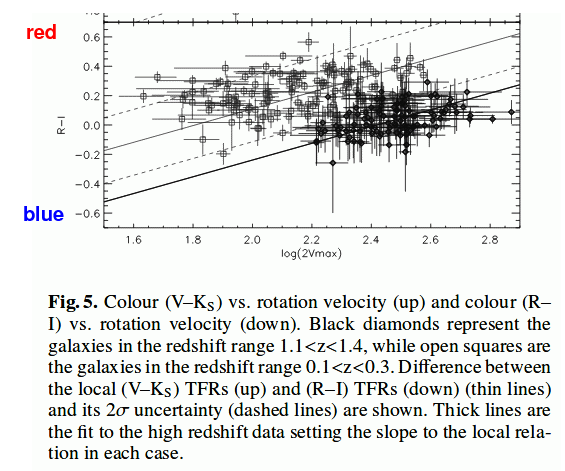
Taken from Figure 5 of
Fernandez-Lorenzo et al., A&A 521, 27 (2010)
It's probably safest to apply the Tully-Fisher method only to galaxies in which the effects of evolution aren't too large; perhaps out to redshifts of z = 0.1 - 0.2, which corresponds to around 500 or 700 Mpc. That's still a very large region!
This story begins in 1976, when astronomers Sandy Faber and Robert Jackson published a paper we will call FJ76. This paper described a set of relationships between the observable properties of elliptical galaxies.
Most elliptical galaxies do not have a significant rotation; that is, the motions of the stars within them show little evidence for a common direction. However, in some galaxies, the stars move very quickly in their orbits -- these tend to be the massive ones -- and in others, the stars move relatively slowly. One way to quantify the motions of stars in such systems is by the dispersion of their velocities: mathematically speaking, if we could measure the radial velocities vi of N individual stars i in a galaxy (which we can't, in almost all cases), the velocity dispersion σ could be calculated as
where ![]() is the average velocity.
is the average velocity.
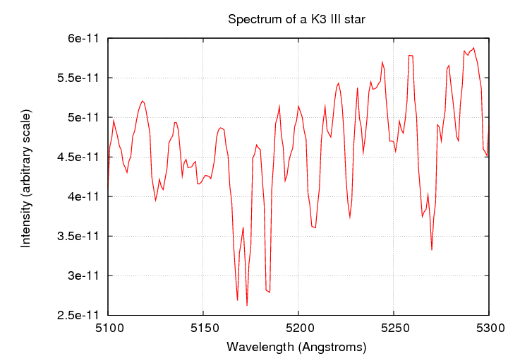
In most galaxies, we can't distinguish individual stars. When we take a spectrum, the light of many, many stars is all mixed up, yielding a composite spectrum of the entire population. Since some of the stars are moving towards us, and others away from us, while some have no radial velocity at all, features in the composite spectrum are smeared out in wavelength space. The larger the range of motions, the larger the degree of smearing.
Consider this single K3 III star, at rest with respect to the Earth. The spectrum is taken from STELIB via Vizier.
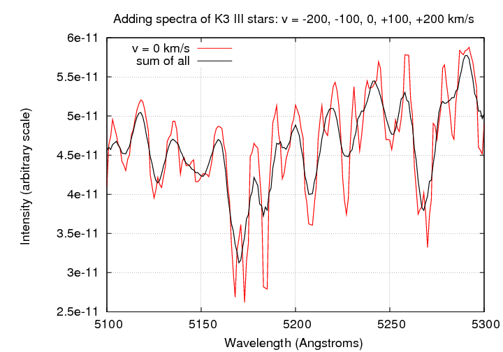
If we add together a set of 5 stars, moving with different radial velocities, then the integrated spectral lines will will look smeared out compared to the original. In a real galaxy, of course, we add together not 5 stars, but millions!
Faber and Jackson measured the velocity dispersion in their sample of elliptical galaxies by comparing the spectrum of light from the center of each galaxy to a series of synthetic spectra, in which a single template spectrum was broadened in a series of steps:

When they compared the velocity dispersion of each galaxy to the absolute magnitude of the galaxy, they found a pretty good correlation: galaxies with large velocity dispersions tend to be more luminous.

Another connection can be made between velocity dispersion and mass-to-light ratio: galaxies with high velocity dispersions also have high mass-to-light ratios. Since velocity dispersion is correlated with absolute magnitude, this means that mass-to-light ratio is also correlated with absolute magnitude.

So, let's summarize the findings of FJ76: elliptical galaxies (*) appear to be a family of objects which are vary in a systematic way, as a function of a single parameter.
(*) aside from dwarf ellipticals
   low mass                                       high mass

   <------------------------------------------------------>

   low luminosity                            high luminosity

   small velocity disperson        large velocity dispersion

   low mass-to-light                      high mass-to-light

   small size                                     large size

   <------------------------------------------------------>
In the years since FJ76, astronomers have accumulated many more observations of elliptical galaxies. We confirm that there is some close connection between several fundamental properties of ordinary elliptical galaxies.
The top-left panel from this figure Diaz and Muriel, MNRAS 364, 1299 (2005) shows a more recent version of the luminosity vs. velocity disperson relationship. It's obvious, but note that there is quite a bit of scatter around the trend. The relationship looks a little bit tighter if one plots luminosity as a function of size, as shown in the panel at top right.
Now, the bottom-left panel shows a rather weak dependence between velocity dispersion and radius: big galaxies have high velocity dispersions. But there might be some sort of systematic skewing: maybe the connection between radius and velocity dispersion does run exactly along the same lines as the connection between radius and luminosity. In that case, we could improve the quality of the relationship by throwing all three quantities into a big blender -- if we mix them up in JUST the right proportion, we can find a model which matches the observations better than the simple one. Look at the bottom-right panel in the figure above.
Because there are three variables, not just two, people describe this relationship among the properties of elliptical galaxies as the fundamental plane (the term was coined by Djorgovski and Davis in 1987). The idea is that we can use any two of the three quantities to predict the value of the third, in some manner equivalent to:

There are many different ways that one can express this idea, given that each quantity can be described in several different ways, and on scales with may be linear or logarithmic. Bernardi et al,, AJ 125, 1866 (2003) show how the relationship between dynamics, luminosity, and size is seen in passbands across the optical.
So, how does all of this help us to find the distance to an elliptical galaxy? Well, if we have carefully measured the properties of many galaxies, we may be able to determine the "constant" in the fundamental plane equation,
and so turn it around to solve for the luminosity of a galaxy:

The terms on the right-hand side are both observable quantities, although each must be defined carefully and in a consistant manner. The velocity dispersion is more difficult to measure, requiring a big telescope to measure the spectrum with decent resolution.
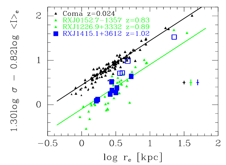
How well does it work? A recent paper, Scott et al., MNRAS 451, 2723 (2015), describes measurements of elliptical galaxies in three relatively distant clusters, averaging z = 0.05. The authors find that if they choose the galaxies carefully, limiting the objects to the most luminous examples, and make a particular set of measurements in a particular way, the scatter in the relative luminosities is pretty small:

Figure 4 from
Scott et al., MNRAS 451, 2723 (2015)
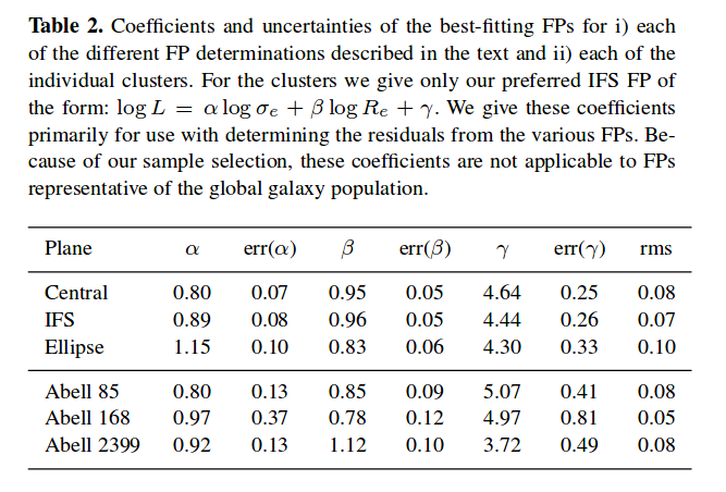
Table 2 from
Scott et al., MNRAS 451, 2723 (2015)
  Q:  Estimate the uncertainty in values of log L from this table.


  Q:  What is the percentage uncertainty in L?


  Q:  What is the percentage uncertainty in relative distances
          computed using such values?
How far away can we use this technique? Well, the good news is that our current instruments can measure these quantities in some elliptical galaxies out to redshifts beyond z = 1.
Taken from Figure 2 of
Fritz et al., AN 330, 931 (2009)
The bad news is the same as that for the Tully-Fisher method: at these large distances, we are looking far enough into the past that the stellar populations in the distant galaxies are considerably different from those in local galaxies. Trying to apply this method will involve some complex adjustment for the changing stellar properties, which makes it less reliable.
Copyright © Michael Richmond.
This work is licensed under a Creative Commons License.