 Copyright © Michael Richmond.
This work is licensed under a Creative Commons License.
Copyright © Michael Richmond.
This work is licensed under a Creative Commons License.
Let's start with a very simple, basic lightcurve for a transit. What are the quantities we measure?
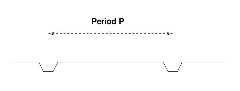
There are two quantities which are immediately obvious:
Oh, and there's one more which becomes available if you have patience:
   Q:  What's the additional property one can
           determine from light curves of transits?
Now, these are only the obvious measureable quantities; if one has very high signal-to-noise ratio, one can learn additional things from the exact shape of the light curve during ingress and egress, and from the shape of the bottom of the light curve.
But, with these these three simple quantities, one can figure out a number of physical properties of the planet and its host star.
Given only the transit light curve observables
let's see what we can figure out about the host star, or its planet, or both. I'll assume that the orbit is circular and (probably) that the planet's mass is much smaller than its host star's mass.
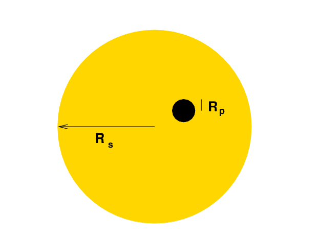
The relative sizes of the host star and the planet are pretty obviously related to the depth.
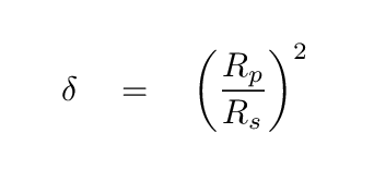
This simple equation glosses over several minor complications; for the full story, see Winn's chapter in "Exoplanets".
If we compare the duration of the transit to the period of revolution, we can find a different ratio involving the radius of the host star, Rs.
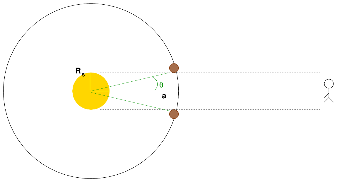
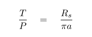
The angle θ shown above can be related to a ratio of distances, but also to a ratio of times.
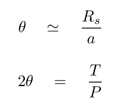
   Q:  Can you derive a connection between the observeable times
             and the (not observable) distances?
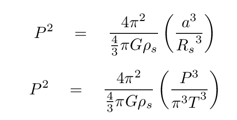
Now, if you take this ratio of stellar radius to orbital radius, and throw it together with Kepler's Third Law, you can end up with an expression for the density of the host star in terms of the observables.
Q: Can you do it?
Now, the very fact that the planet passes in front of its star requires that the inclination of the orbital plane to the line of sight be close to ninety degrees; so, for some purposes, one can declare that the inclination angle must be ninety degrees and be done with it. But that's not strictly true, and, if one wishes, one can place formal constraints on the inclination with some complicated work; see Winn's chapter in "Exoplanets".
In some situations, one can measure the radial velocity variations of the host star, in addition to observing transits. When you have extra information, what additional parameters can you derive?
It is somewhat disappointing to find out that, even with the velocity information, one still cannot compute the mass of the planet alone. Rats.
Some very ingenious people figured out that the combination of transit and radial velocity measurements can be used to compute the surface gravity of the planet. Wierd, but cool. Again, for the details, see Winn's chapter in "Exoplanets".
If you look at a transit at different wavelengths, you'll see that its shape changes slightly. The figure below shows the transit of a planet around the star HD 209458 at wavelengths ranging from about 3000 Angstroms (purple, at bottom) to about 1000 Angstroms (red, at top).
![]()
Image taken from Figure 3 of
Knutson et al., ApJ 655, 564 (2007)
   Q:  What is the major difference between the shape
       of the curve at short vs. long wavelengths?
Yes, that's right: the transit light curve has a
It's the same star in each case -- so why the difference?
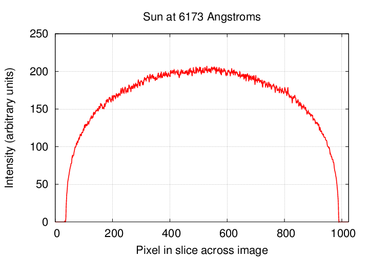
Well, take a look at this picture of the Sun.
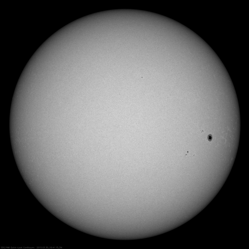
Image of the Sun at 6173 Angstroms taken 3/30/2015
from the
Solar Dynamics Observatory website
The solar disk is clearly NOT the same brightness across the entire face; instead, it's brighter near the center, and fades away toward the edges. Astronomers call this limb darkening. You can read more about limb darkening here.
One important feature of limb darkening is that it depends on the wavelength at which one observes: shorter wavelengths lead to stronger limb darkening.
The dip in light created by a transit shows us a sort of mirror image of the surface brightness of the star: the dip is deeper where the surface is brighter.
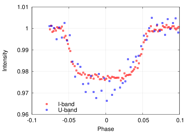
Transits of WASP 39 measured by
Ricci et al., PASP 127, 143 (2015)
Careful measurements of the transit at multiple wavelengths allow astronomers to determine the degree of limb darkening in a planet's host star; and that, in turn, can help them to pin down properties of the host star.
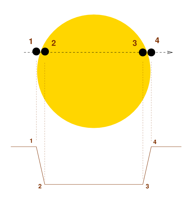
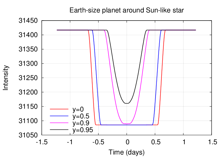
But beware the possible confusion between limb darkening and off-center transits. Even long-wavelength observations can yield transits with rounded bottoms, if the planet happens to cross its host star above or below the center of the disk. Consider four possible transits of a single star:
![]()
These four paths of the planet in front of its star would produce four rather different transit light curves:
You all know the story of the discovery of Neptune, right? Right?
If not, you can refresh your memory:
The basic idea is that careful and repeated observations of one visible planet can reveal small changes in its motion which can be explained by the presence of a second invisible planet. In the case of Neptune, astronomers noticed small discrepancies between the observed and predicted locations of Uranus in its orbit, during a single revolution around the Sun.
In the case of exoplanets, we can't really "see" any planets directly, but transits allow us to measure VERY precisely the position of one planet at a particular time; or, if we observe many transits, at many times. We can make a model of the orbit of this transiting planet around its star, and use the model to predict the times of future (or past) transits. IF any other planets happen to orbit the same star, their gravitational influences might cause the transiting planet to arrive a little earlier each time -- or maybe a little later each time.
All you have to do is to measure the time of several transits very, very carefully. It sounds easy -- but in practice, it's pretty difficult.
Let's take a look at one particular example: Hoyer et al., ApJ 733, 53 (2011) measured 5 transit times of OGLE-TR-111b themselves, and combined their data with 11 other measurements from the literature.
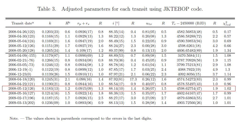
Table 3 taken from
Hoyer et al., ApJ 733, 53 (2011)
   Q:  What is the precision of the times in this table?
             Pick the event inside the box as an example.


   Q:  Why is the precision so low?  Shouldn't it be possible
             to measure the time more precisely?
Well, let's look at a few of the measurements:
![]()
A portion of Figure 5 from
Hoyer et al., ApJ 733, 53 (2011)
A few things are pretty clear from these curves:
But there are additional factors, too:
The figure below illustrates the difficulty of determining the time of a transit. It shows the difference between the times computed by two groups, starting with exactly the same light curves.
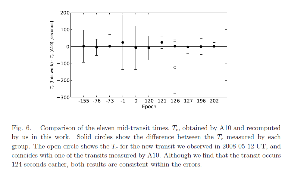
Figure 6 from
Hoyer et al., ApJ 733, 53 (2011)
The bottom line is ... this sort of measurement is difficult. In the case of OGLE-TR-111b, there appear to be no significant variations in the times of transits. The authors can only place limits on the existence of other planets in the system. Note the especially stringent limits which occur at certain locations in the host system.
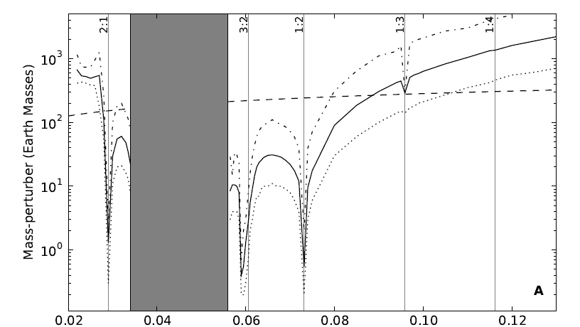
Figure 9 from
Hoyer et al., ApJ 733, 53 (2011)
If we see a planet passing in front of the star, there's a very good chance that the planet will also pass BEHIND the star half a period later. Different authors use different words to describe these events:
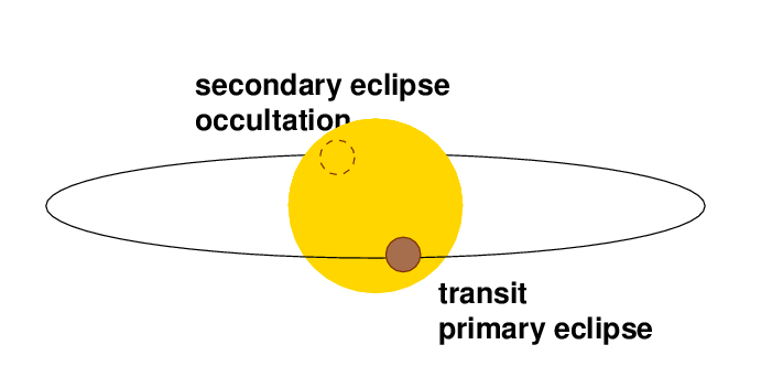
I'll choose the term occultation to refer to the times when the planet is hidden behind its host.
In theory, the system as a whole should appear fainter during an occultation; after all, the planet is producing SOME light which travels in our direction. Now, that light could have two sources:
In the great majority of cases, the planet's contribution to the total light is so small that we can't detect the tiny drop during an occultation. Rats.
But in a few cases, we CAN measure that drop, and it can tell us something extra about the planet.
For example, Hu et al., ApJ 802, 51 (2015) look at the occultation of two systems in visible light.
Q: Guess which instrument they were using
Yes, Kepler, of course: it's the only instrument (I think) sensitive enough in the optical to see the effect of occultations. The authors point out that the appearance of a planet in reflected light depends on the properties of its surface and atmosphere:
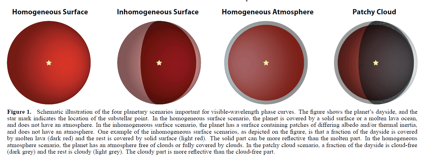
Figure 1 taken from
Hu et al., ApJ 802, 51 (2015)
Let's look at the measurements of the occultation in the system Kepler-7b. In both panels, the black symbols are the measurements.
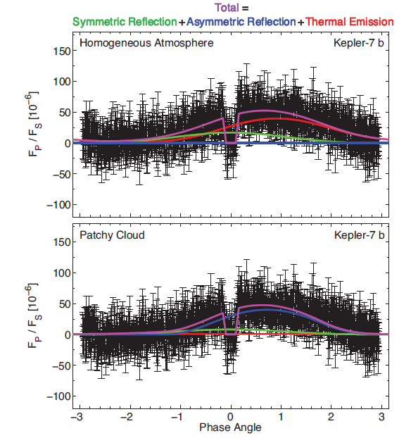
Figure 2 taken from
Hu et al., ApJ 802, 51 (2015)
   Q:  Is there an asymmetry in the light curve?


   Q:  What could cause such an asymmetry?
Hu et al. show that their observations can be equally well fit by two models:
The first possiblility, shown by the curves in the upper panel, is an atmosphere which heats up during the day. The gas will be warmest not at local noon, but some time afterward. Thus, the brightest location on the planet will be slightly offset from the sub-solar point. We will see the planet appear brightest to us when this hot spot is pointed nearly at us, which will occur a short time before or after the occultation.
What a minute -- did I say "thermal emission?" Well, maybe I only implied it, but still -- can we SEE thermal emission with Kepler? Let's check:
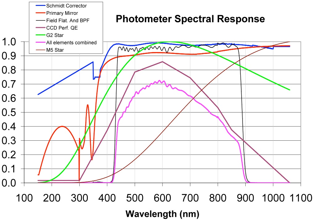
Yowza. The Kepler detectors stop responding at about 900 nm, which isn't normally what I would consider part of the "thermal infrared" ... but I guess when one is dealing with parts per million, maybe it is.
However, the authors go on to point out that although their own Kepler data can be explained by either thermal emission or reflection from clouds, other observations by Kepler and Spitzer are inconsistent with the "thermal emission" possibility. Thus, it looks like Kepler-7b has some big patches of clouds.
Detecting occultations can also be done in the near-infrared, where the planet's thermal emission will become more important relative to reflections of the host star's light. Let's begin with measurements by Spitzer of the planet WASP-5b, as described by Baskin et al., ApJ 773, 124 (2013) . As you can see, even with a space-based observatory working in the near-IR, detecting these occultations is not a walk in the park.
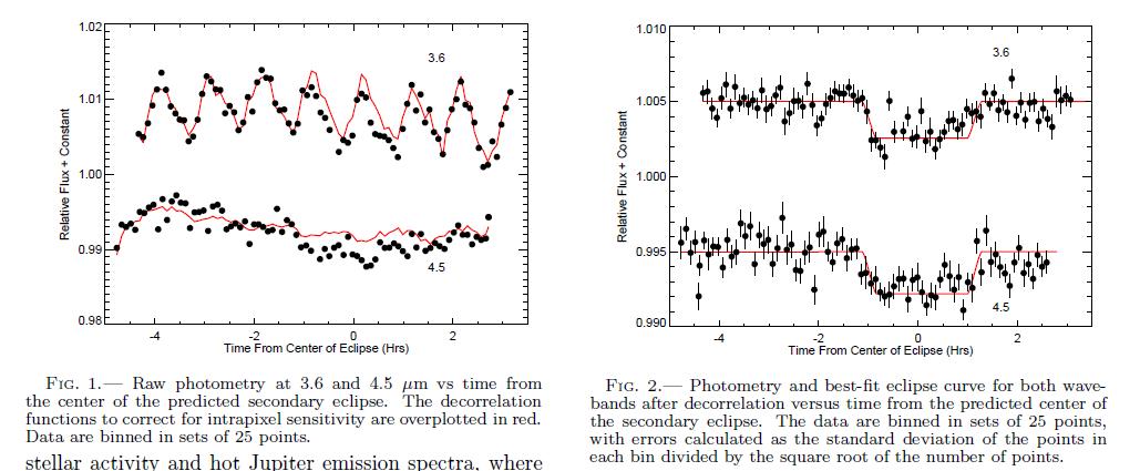
Figures 1 and 2 from
Baskin et al., ApJ 773, 124 (2013) .
What can we learn from these tiny little dips as the planet hides behind its star? One measured quantity here is the ratio of planetary to stellar flux at certain wavelengths. One can make models of planetary atmospheres (or surfaces) which can be compared to this measured ratio.
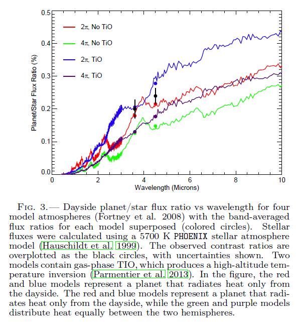
Figures 1 and 2 from
Baskin et al., ApJ 773, 124 (2013) .
Another measured quantity is the time of the occultation. If the planet's orbit is circular, the occultation will occur exactly halfway between transits. But if the orbit is elliptical, there can be an offset. In the case of WASP-5b, Baskin et al. find the occultation occurs 3.7 +/- 1.8 minutes away from the mid-point between transits; they conclude that the orbit is very likely circular.
Hmmm. There's one little item that might complicate this analysis, if we don't include it.
    The mass of the host star in this system is M = 1.276 solar.
    The period of the transiting planet is P = 4.95466 days.

    Q:  What is the star-planet separation a?


    Q:  How much time does it take for light to reach us
           from an occultation than a transit?
Believe it or not, an occultation in at least one exoplanet system has been observed in the near-IR from the ground! And, even better, it's the same system -- WASP-5b -- which was observed with Spitzer, as mentioned above. Chen et al., A&A 564, 6 (2014) used the MPG/ESO 2.2-meter telescope and GROND instrument to measure WASP-5b in J, H, K bands simultaneously. As you might expect, this project pushes the envelope of ground-based observations.
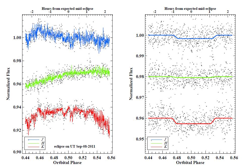
Figure 2 taken from
Chen et al., A&A 564, 6 (2014)
It helps the eye if one bins the data.
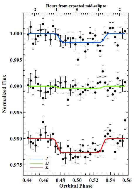
Figure 2 taken from
Chen et al., A&A 564, 6 (2014)
What can you do with these measurements? Well, as before, the measured quantity is the ratio of planet-to-star intensity. One can create models of this quantity for various types of surface or atmospheric properties, and compare the models to the observations.
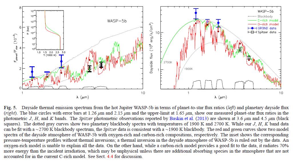
Figure 5 taken from
Chen et al., A&A 564, 6 (2014)
In this particular case, there is a bit of a discrepancy between the ground-based measurements of Chen et al., A&A 564, 6 (2014) (shown with blue symbols) and the space-based Spitzer measurements of Baskin et al., ApJ 773, 124 (2013) (shown with hollow black squares).
Well, this is a very tough observational project, so it shouldn't be surprising that the results are still uncertain.
Copyright © Michael Richmond.
This work is licensed under a Creative Commons License.